How to Switch First and Last Name in Excel

Data manipulation is one of the most powerful abilities of Excel. Flash Fill is a tool in Excel that enables you to manipulate data in a cell according to your needs.

In this tutorial, we will learn how to switch first and last names in Excel with the help of Flash Fill.

Switch First and Last Name

Now we will walk through the steps of switching the first and last names in Excel, and we will use Flash Fill for this purpose.

Flash Fill works as follows: you define a new pattern, and Flash Fill imitates this pattern for all other cells. In this case, the pattern that we will create is going to be “LastName, FirstName”.

Step 1: Go to a cell that contains a full name. In the cell right next to it, write the pattern you want in a reverse fashion: “LastName, FirstName”.

Write the new pattern with swapped full name

Be careful that the first and last names are written correctly, just like the original cell.

Step 2: Press Enter on your keyboard to go to the cell below, or click on the cell below the new pattern.

Go to the cell below

Step 3: In the Home tab, click on the Fill icon in the Editing part in the Excel ribbon, and then click on Flash Fill.

Click on Fill and then Flash Fill

This will automatically fill out all cells next to a full name, and your names will successfully be switched:

Full names swapped

Using this method, you can use any pattern that includes a first name and a last name. For example, you can also abbreviate a first name:

First name abbreviated with Flash Fill

As long as you provide a new name format, Flash Fill will automatically learn the pattern and apply it to other cells. It’s like magic, right?

This extremely easy method can enable you to perform all kinds of text manipulation. Learning to use Flash Fill is an excellent skill. Nice job!

You may want to check how to separate or combine first and last names in Excel and then sort by last name in Excel.

How to Save an Excel Table As an Image

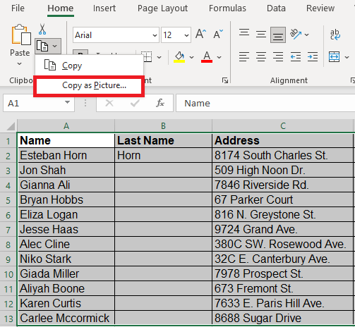
Excel is a great way to store, compute, and sort information; however, there may be times when you want to save the tables in Excel as images for use on the web, brand print material, or for training.

Use the Copy Feature in Excel to Save an Excel Table as an Image

  1. Highlight the table that you want to save as an image.
Image showing a highlighted table in Excel.

  1. Click the down arrow next to the Copy button in the Clipboard group and click the “Copy as Picture…” selection.
Image showing the Copy As Picture option in Excel.

  1. Open up your favorite image editor. You can use Paint™, Paint 3D™, Photoshop™,  GIMP™, or Photos™ on Mac™. For this tutorial, we will use Paint™.
Image showing a blank canvas in Paint.

  1. Click the Paste option in Paint, and the image appears on the canvas.
Image showing the Paste option in Paint.

  1. Resize the canvas by moving the small white rectangles on the canvas with the mouse so that they match the size of the picture.
Image showing the Canvas resizing handles in Paint.

  1. Edit the image as needed and save the file.
Image showing an Excel table pasted into Paint with the canvas cropped to size.

Use the Print Screen Button to Save an Excel Table as an Image

  1. Open the worksheet you wish to save as an image and press the Print Screen (PrtScr) button on your keyboard.
Image showing a worksheet table in Excel.

  1. Open a new canvas in your image editing software, and press CTRL + V or CMD + V if you use a Mac.
Image showing a portion of the Paint application in Windows.

  1. The screenshot will appear on the canvas and will need editing to isolate the Excel table from the complete image.
Image showing Excel table pasted into Paint after  Print Screen shortcut.

Note: if your keyboard does not have a Print Screen button, Windows users can use the Fn + Windows Logo Key + Space Bar combination to take a screenshot. Mac users can take a screenshot with CMD + Shift + 3 together.

Use Shortcut Keys to Save an Excel Table as an Image 

  1. Once your worksheet is open in Excel, press CTRL + C or CMD + V for a Mac to store the picture in the computer’s memory.
Image showing a worksheet table in Excel.

  1. Open your image software and press CTRL + V or CMD + V on a Mac to paste the picture on the blank canvas.
Image showing Excel table pasted into Paint after Print Screen shortcut.

  1. Edit the picture to fit your needs.
Image showing an Excel table pasted into Paint with the canvas cropped to size.

Conclusion

Now you have discovered the different methods for saving an Excel table as an image. Explore the many other topics on our blog to continue increasing your knowledge of Excel.

You can also save the data or workbook without formulas if you want another option of saving the Excel table.

How to Remove Hyperlink in Excel?

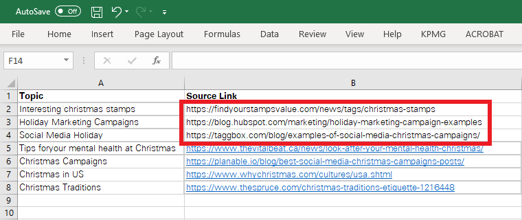
Have you ever imported data to Excel from an external source with many unwanted hyperlinks that came along?

Also, you might have come across multiple undesired hyperlinks automatically generated by Excel for emails and URLs inserted into a workbook.

Unwanted hyperlinks can cause undue trouble. Every time you select a cell containing a hyperlink, excel would automatically redirect you to the destination link.

Hyperlinks that are not needed can be removed from Excel with sheer ease.

Continue reading to know how you can instantly remove hyperlinks in Excel.

To better learn the easy two-step process of removing hyperlinks from selected cells in Excel, let’s stipulate an example below.

The data set below collates different links containing information relevant to various topics. As soon as the links are input, Excel recognizes them as hyperlinks and formats them into blue color and underlines them.

Dataset containing multiple hyperlinks in Excel

To remove the hyperlinks from only some selected cells, here are the steps that you need to follow.

Step 1:

Select the cells containing the hyperlinks that you want to be removed.

Selection of cells containing hyperlinks to be removed

Step 2:

Right-click by keeping the cursor on the selected cells to see the pop-up menu as below.

Right-clicking on the selected cells to see the pop-up menu

From the pop-up menu that opens up, select the option, ‘Remove Hyperlinks’.

Selection of the option ‘Remove Hyperlinks’

Excel removes hyperlinks from the selected cells as evident below.

Hyperlinks removed

That is it. Removing hyperlinks from Excel is only that easy.

However, what if you have an Excel file that is densely packed with hyperlinks? Is it not hectic to select each cell to remove the hyperlink therefrom? It definitely is. Here is a shortcut that may help you with it.

Continuing with the same example stipulated above, to remove hyperlinks from the entire spreadsheet at the same time, follow the steps below.

Step 1:

Press ‘Ctrl+A’. This is the shortcut to select all the contents of an active sheet.

Selection of all the contents of a workbook

Step 2:

Right-click against the selected cells to have the pop-up menu opened. Opt for ‘Remove Hyperlinks’ as follows.

Removing hyperlinks from the entire spreadsheet

Excel removes hyperlinks from the entire spreadsheet as follows.

Hyperlinks removed from the entire spreadsheet
Pro Tip: Prevention of Automatic Navigation to the Destination Link

As soon as you select a cell that contains a hyperlink, you will be navigated to the destination link. Or in case of an email address, Excel would present you with the option to send an email to the subject address.

If Excel redirects you to the destination link automatically upon selecting a cell, you may turn it off as follows.

File > Options > Advanced > Editing options

Check the option for 'Use CTRL + Click to follow hyperlink'. Once this is done, Excel would present you with the option to press ‘Ctrl’ to follow a link. Merely selecting a cell in Excel wouldn’t navigate you to the destination page.

Suggested Tutorial: How to Extract URL from Hyperlinks in Excel

It is often the case that you’ve to work with Excel files containing excessive Hyperlinks. For example, the Human Resource department of a Company may have to maintain a record for all of its employees, including their names, numbers, and email addresses.

Whenever fed into Excel, email addresses are recognized by Excel as hyperlinks. If you don’t want the file to contain hyperlinks, such settings of Excel might prove problematic. This is because every time you feed the details of a new employee into the Excel sheet, Excel would automatically turn the email address into a hyperlink.

Removing each hyperlink time and time again is time-consuming and frustrating. To prevent Excel from generating hyperlinks automatically, you can disable the same from the settings. Here’s how you can do it.

Step 1:

Go to File > Options as follows.

File > Options

Step 2:

Selecting options would open up a window of Excel options as follows.

Excel Options

From the said window, choose Proofing > AutoCorrect Options as highlighted above. This would open up a pop-up window.

ChooseAutoFormat as you type and uncheck the box for Internet and network paths with hyperlinksas highlighted below.

Automatic hyperlinks turned off.

This will turn off the automatic hyperlinking within Excel. Now, as you type or Copy / Paste links in Excel, those would remain as text, and Excel would not automatically turn them into Hyperlinks.

Pro tip: This setting will be applied to the entire Excel application. Any workbook that you create or edit with Excel will have the same settings applied.

However, after these settings are applied, you can still add hyperlinks to one or more cells by right-clicking on the desired cell. From the pop-up menu that then opens up, select ‘Link’. This would open up a dialogue box where you can insert the destination link to be added as hyperlink to that cell.

Conclusion:

Hyperlinks make an intelligent feature of Excel. However, undesired hyperlinks are often a nuisance. Hope this article helped you learn all that you needed to know how to remove hyperlinks in Excel.

How to Combine First and Last Name in Excel

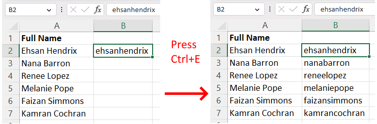
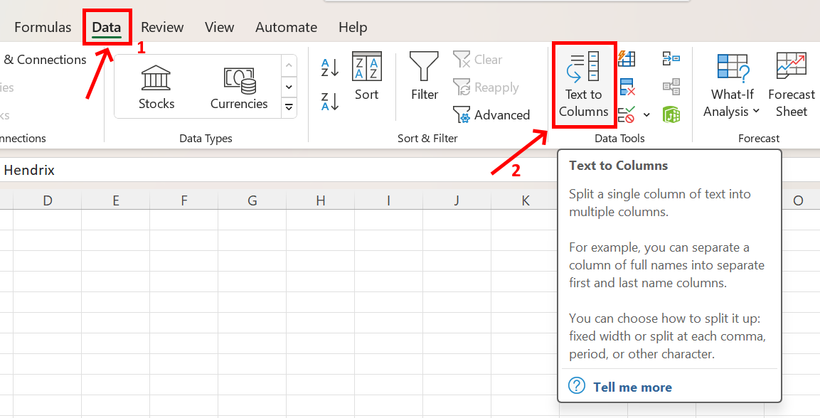
Excel has many useful functions and tools that enable us to perform text manipulation. That’s why, when you have first and last names in separate columns in a spreadsheet, it’s extremely easy to combine them into a full name, whether you want it separated with a space or a comma.

In this tutorial, we will learn how to combine first and last names in Excel using the CONCATENATE function, the ampersand (&) operator, and Flash Fill.

Using the CONCATENATE Function to Combine First and Last Name

The CONCATENATE function enables us to combine multiple cells or values. We can use this function to combine first and last names and separate them with a space or a comma. Let’s learn how…

Write the following formula in a new cell to combine first and last names with a space:

=CONCATENATE(A2, " ", B2)

The first cell name (A2) refers to the first name, and then we concatenate the space character (“ “), and the last name (B2).

Use CONCATENATE to combine with space

You can drag the small green rectangle in the bottom right of the cell with the formula, and drag it downward to apply the concatenate operation to other cells.

Drag downward to apply concatenate to other cells

If you want to combine the names with a comma with the format “LastName, FirstName”, use the following formula:

=CONCATENATE(B2, ", ", A2)
Use CONCATENATE to combine with comma

The CONCATENATE function can combine multiple text values or cells. Therefore, it can also be used to combine a first name, middle name, and last name:

=CONCATENATE(A2, " ", B2, " ", C2)
Combine middle name with CONCATENATE

So, the trick is: to write all the cell values and separators inside the CONCATENATE formula and separate them with commas. When you learn this simple formula, you can combine anything!

Using the Ampersand (&) Operator Function to Combine First and Last Name

Text combination can also be achieved with the ampersand (&) operator. Write the following formula to combine first and last names with a space:

=A2&" "&B2
Use ampersand to combine with space

If you want to combine the names with a comma, type the following formula in a new cell:

=B2&", "&A2
Use ampersand to combine with comma

The ampersand operator (&) works as follows: you need to start the formula with the equal (=) sign, and then write the cell names and separators, and type ampersand (&) between each of them. This is another elegant way of combining first and last names.

Using Flash Fill to Combine First and Last Name

Without using operators and formulas, it is perfectly possible to combine first and last names: with the help of Flash Fill. Flash Fill is a tool that learns and applies patterns. Follow the steps below to combine using Flash Fill.

Step 1: Next to the first and last names, write the full name in a new cell.

Write full name in a new cell

Step 2: Go to the cell below by pressing Enter, or clicking on the cell.

Go to the cell below

Step 3: In the Home tab, click on the Fill icon in the Excel ribbon, and then click on Flash Fill.

Click on Flash Fill

Flash Fill will automatically learn the pattern, and combine the first and last name for all cells.

Flash Fill combines all names

You can apply the same steps if there are middle names in your data. As long as you type the full name exactly as in the original cells that contain the first, middle, and last names, the combination pattern will be learned and applied by Flash Fill.  

In this tutorial, we learned how to combine first and last names in Excel using the CONCATENATE function, the ampersand (&) operator, and Flash Fill. You can choose whichever method suits you best.

You may want to check how to switch first and last names in Excel or sort by last name in Excel.

How to Insert Square Root Symbol in Excel

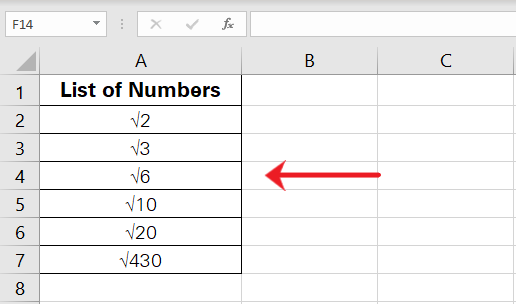
Before anything, what is a square root symbol? Let me quickly take you back to high school mathematics. Here’s what the square root symbol looks like.

We often need this symbol in your spreadsheets for a variety of tasks. Some of the time to compose a formula, write down an expression, and so much more.

How do you add that in Excel? There are multiple ways how you can do that. Let me take you through all of them in the article below.

Also if you wonder how to add other symbols, you can check our other articles:

Copy/Paste the Square Root Symbol in Excel

Out of many ways to add the square root symbol in Excel, the first and the easiest is to copy it from below simply.

  1. Select this square root symbol √.
  2. Right-click on it > Click on Copy.
  3. Go to the relevant cell in your Excel sheet.
  4. Double-click on the cell to activate it.
Activation of cell

  1. Right-click to launch the Paste Special Options.
  2. Click on Paste as shown below.
Paste options

And there you go.

Square root symbol pasted

Ta-da! The symbol is pasted to your Excel sheet. Make as many copies of the same as desired, and you’re all set.

However, this method is only advisable if you only need to add one (or a very few) square root symbols to your sheet. If you need them more than that, try the other methods discussed below.

Insert Square Root Symbol Using Symbol Option

The square root is recognized as a symbol by Excel and is included in the symbols library of Excel. Let’s find it out together.

  1. Activate the cell where you want the square root symbol inserted.
  2. Go to the Insert Tab > Symbols as shown below.
Select Symbol from Symbols

This will launch the Symbol dialog box as follows.

Symbol dialog box

  1. Set the Font to normal text (as shown below).
  2. Set the Subset to Mathematical Operators (as shown below).
Font and subset setting

From the signs that appear, select the “Square Root” symbol.

  1. Click on Insert.

And there, you have it added to your sheet.

Square root symbol added

The next time you need to add it, it will be saved in the recently used symbols, so the whole process gets quicker.

Recently used symbols

Pretty cool, right?

Insert the Square Root Symbol Using the UNICHAR Function

Another method you can use to add the square root symbol to an Excel sheet is by using the UNICHAR function. How? Let’s see that below.

TIP!

The UNICHAR function works with ASCII codes (which are numerical values). For each of these codes, the UNICHAR function returns a unique code. 

Inserting the square root symbol using the UNICHAR function is simple if you know the required ASCII code. And that code number is 8730. Let’s now see how to use it to insert the square root symbol in Excel.

  1. Activate the cell where you want the square root symbol inserted.
  2. Begin writing the UNICHAR function as follows:

= UNICHAR (

  1. Write in the code 8730 as follows:

= UNICHAR (8730)

the UNICHAR code

  1. Hit Enter to see the results below.
UNICHAR returns the results

See that?

However, there’s one problem with the UNICHAR function. It does add the square root symbol, but if you want to use it with other characters, you will have to concatenate it with them.

Like below.

UNICHAR with concatenate

To help this, you can copy and paste the square root symbol as a simple value. Here’s how to do it.

  1. Copy the formula.
  2. Go to another cell and right-click to launch the Paste Special options.
  3. Paste it as Values.
Copy pasting as values

Check out the formula bar to see that the UNICHAR formula has gone away. What’s left behind is a simple square root symbol.

UNICHAR pasted as values

Now you can easily use it around your spreadsheet without worrying about the UNICHAR formula running behind it. How cool is that?

Insert the Square Root Symbol Using a Keyboard Shortcut

It’s always easier to simply use your keyboard to type any character, and the square root symbol is no exception.

Although you will not find the square root symbol on your keyboard, you can still type it using the following keyboard shortcut.

What is that? The Alt key + 2 + 5 + 1.

All of these 4 keys are to be typed in succession, i.e., one after the other.

TIP!

Here’s something very important that you must know about using this keyboard shortcut. This keyboard shortcut will only work with a numeric keypad.

So if your keyboard (or laptop) doesn't have a numeric keypad, this keyboard shortcut would not work with the other number keys on your keyboard. In this case, you'd have to use any of the methods discussed above.

Let us now quickly go through the steps to be followed to insert the square root symbol using this shortcut.

  1. Activate the cell where you want the square root symbol inserted.
  2. Press the following keys on your keyboard in sequential order.

Alt key + 2 + 5 + 1

Keys to be pressed

And that’s it. You have it inserted in the selected cell.

The square root symbol

Change the Format of Values to Add the Square Root Symbol

This method comes last because it works differently than the other methods on this list.

Under this format, we only change the format of the values in our spreadsheet to prefix them with a square root symbol. So, in essence, you don’t add the character to your sheet. But the values in your sheet are formatted as such to exhibit it.

Let’s change the format of the values in the image below to see how we can do it.

List of Values

Here are the steps to be followed.

  1. Select all the cells where the square root symbol is to be added.
Selection of cells

  1. Go to the Home tab > Number > the small arrow button to launch the Format Cells dialog box.
Format Cells dialog box

  1. From the Format Cells dialog box, go to the Number Tab.
  2. Go to “Custom” from the pane on the left.
  3. Add the square root symbol ( √ ) before the category General.
Square root symbol before General

TIP!

You can simply copy it from here ( √ ) and paste it there. Or, if you have a numerical keypad, use the Alt key + 251 shortcuts to add one instantly.
  1. Click on Okay. A square root symbol will be added before every number on the list.
Square root symbol added

However, these numbers are only formatted to include a square root symbol. A square root symbol doesn’t actually exist in the cell.

This is evident from the Formula bar.

Formula bar

Hence, this method is only suitable if you want the square root symbol for presentation purposes.

Conclusion

In this guide, we explored different ways of inserting the Square root symbol in Excel. We saw the technique of using UNICHAR function, we saw how to use formatting to insert the symbol, and we also tried some cool keyboard shortcuts.

You can use any of the above explained methods to insert Square root in Excel. It might take you some practice before you master the art, but once you do, it will seem easier than falling off a log.

Our favorite method is using the UNICHAR function to add the symbol – have you found yours? If not, then what are you waiting for? Find the best suited method for your purpose now!

How to Separate First and Last Name in Excel

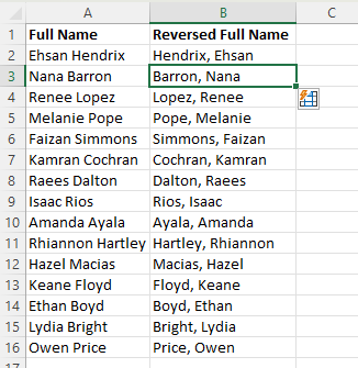
Let’s say you have a spreadsheet with lots of names, and you want to make an analysis of the data.

When the first and last names are together in a cell, it makes it extremely difficult to analyze, sort, and find important information.

To eliminate this difficulty, we will learn in this tutorial to separate first and last names in Excel and also will learn how to separate a name that’s separated with a space, or a comma.

Separate First and Last Name

Splitting a full name into first and last names is extremely easy in Excel with the help of the Text to Columns feature. Let’s learn how…

Step 1: Choose the cells that contain a full name.

Choose cells with full name

Step 2: In the Excel ribbon, go to the Data tab, and then click on Text to Columns.

Click on text to columns in Data tab

The Text to Columns feature splits a single cell into columns when you choose a delimiter (separator) such as a space, tab, or a comma.

Step 3: In the Convert Text to Columns Wizard, choose the Delimited data type, and click on Next.

Choose the delimited data type and press Next

Step 4: Under the delimiters list, choose Space if the first and last names in your data are separated with a space. Then, click on Next.

Choose space as the delimiter and press Next

When you choose space, the Convert Text to Columns Wizard will automatically give you a preview of the separated data under Data preview. This way, you can make sure that the data will be separated correctly.

Step 5: In the last step, you can select the data format of the newly generated columns. In the case of names, the General data format is perfectly suitable.

In addition, you can select the destination of the separated first and last names.

If you don’t specify a new destination, the separation will be made in place (will override your data). Instead, click on the upward arrow under Destination, and choose the destination cell.

Choose destination cell for separated names

Step 6: After completing all steps, click on Finish.

Perfect! Now, all the full names in your spreadsheet will be split into separate columns as first name and last name:

Full name split into separate columns

If your full names are separated with a comma, you only need to change the delimiter you selected in.

Go to Step 4. Let’s assume the format of your full name is: “LastName, FirstName”.

Full names separated with a comma

To separate full names with a comma, instead of Step 4, choose the Comma separator under the Delimiters list, and then click on Next:

Choose comma as the delimiter and press Next

The rest of the steps are identical. This way, your data can more easily be analyzed:

Full name separated with comma split into separate columns

In this tutorial, we learned how to separate first and last names with a space or a comma in Excel with the assistance of the Text to Columns feature.

Also, you may want to check how to combine or switch first and last names in Excel and then sort by last name in Excel.

Related Tutorial: How to remove the middle initial from the full name

How to Delete Multiple Sheets/Tabs in Excel at ONCE

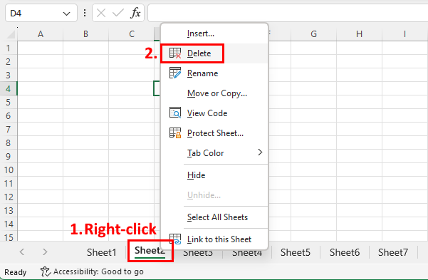
Opening sheets for different purposes within an Excel document is an excellent feature. However, sometimes you may accidentally open multiple unnecessary sheets, which can cause redundancy, especially if you don’t know how to delete multiple sheets in Excel at once.

In this tutorial, we will learn how to delete a single sheet and then to delete multiple sheets simultaneously. This way, you can clean your document from unnecessary sheets with a single click!

Delete a Single Sheet

To delete a single sheet, right-click on the name of the sheet you want to delete, and then click on Delete.

Right click and delete a single sheet

This will successfully delete a single sheet:

A single sheet deleted

Delete Multiple Sheets

If you have more than one sheet you want to delete, you first need to select all sheets you want to delete.

  • If the multiple sheets you want to delete are consecutive, first click on the name of the first (leftmost) sheet. Then, while pressing Shift on your keyboard, click on the last (rightmost) sheet you want to delete. This will select all sheets in between.
Select consecutive multiple sheets with Shift

  • If the multiple sheets you want to delete aren’t consecutive, click on the sheets individually while pressing Ctrl on your keyboard.
Select non consecutive multiple sheets with Ctrl

After selecting the sheets you want to delete, right-click on a sheet name within your selection, and click on Delete.

Right click and delete multiple sheets

This way, multiple sheets are deleted in an instant!

Multiple sheets deleted

In this tutorial, we learned how to delete a single sheet and multiple sheets at the same time.

Related Tutorials: 

Delete a Comment in Excel

Sum Across Multiple Sheets in Excel

How to Sort by Date in Excel

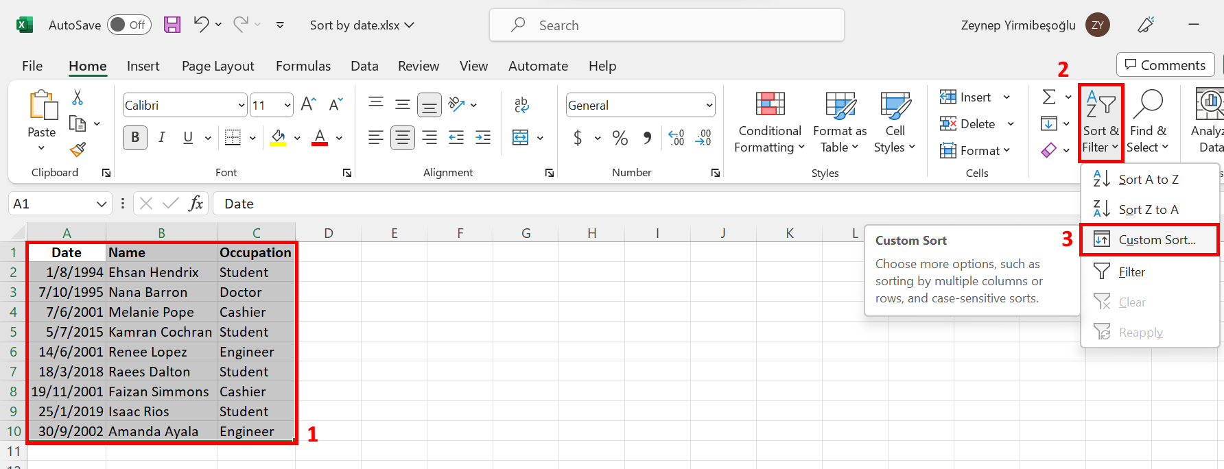
Sorting is an extremely useful function of Excel. Excel sort enables many options and variations so that you can sort your data with any specification.

In this tutorial, we will learn how to sort by date in Excel: we will sort a single column or the entire data by date, and also learn how to perform custom sort.

Sort a Single Column by Date

If your dates are only in a single column, sorting by date is very straightforward. Let’s start…

Step 1: Select the dates in your column.

Select the date cells to sort

You can also select the entire column by clicking on the column name. Just make sure to remove any duplicates from that column.

Step 2: Click on Sort & Filter, which is on the top right of the Excel ribbon.

Step 3: If you want to sort lowest to highest, click on Sort A to Z.

Sort the dates lowest to highest

This will sort the dates in an ascending fashion (lowest to highest):

Dates sorted ascendingly

If you want to sort from highest to lowest, click on Sort Z to A.

Sort the dates highest to lowest

This will sort the dates in a descending fashion (highest to lowest):

Dates sorted descendingly

This method works perfectly if the data you want to sort is independent of other cells or columns. Otherwise, you need to learn how to sort more than one column or the entire data.

The next section covers this case.

Also Learn: How to Sort by Last Name in Excel

Sort Entire Data by Date

Let’s say your data is spread over multiple columns, and you want to sort by date. If you sort by only selecting the date cells, the rest of your data will not be sorted, and irrelevant cells will stay in irrelevant rows. That’s why the sort selection needs to be extended to preserve data integrity.

Follow the steps below to sort your entire data by date.

Step 1: Select the column that contains the dates.

Step 2: Click on Sort & Filter, and then Sort A to Z or Sort Z to A.

Select date column and then click on sort

Since there’s data in other columns, a pop-up will appear:

Step 3: While the “Expand the selection” option is selected, click on Sort.

Expand sort selection pop-up

Now, the entire data is sorted. As can be seen from the image below, the cells in the Name and Occupation columns followed the date cells. This way, you preserved the integrity of the data and successfully sorted it by date.

Entire data sorted by date

Sort Using Custom Sort

If the sort operation that you want to perform is more sophisticated than just sorting by date, then you can use Custom Sort. Custom Sort enables sorting on multiple columns and prioritizing the columns. Let’s see an example.

Step 1: Select the data you want to sort.

Step 2: Click on Sort & Filter.

Step 3: Click on Custom Sort…

Click on custom sort

The custom sort window will appear. In this window, you can choose:

  • Column: which column to sort on (Date, Name, or Occupation)
  • Sort On: which property to sort on (Cell Values, Cell or Font Color, Conditional Formatting Icon)
  • Order: A to Z (ascending), Z to A (descending), or Custom List
Select which column to sort on

If you check the “My data has headers” option, the header row (first row of each column) will not be included in the sort (freeze the header row if you want).

If you want to sort on multiple columns, you can click on “Add Level”:

Sort on two columns including date

Whenever you add a new level, you can choose the options mentioned above (Column, Sort On, and Order). In this example, we will first sort the Occupation column from lowest to highest.

Then, we will sort on the Date column from lowest to highest. The result is as follows:

Data sorted on two columns

Custom sort has first sorted the data with respect to occupation, then within each occupation, sorted with respect to the date. This is a more sophisticated version of sorting by date and shows the power of Excel.

Conclusion

In this tutorial, we learned how to sort data by date in Excel. We learned about different scenarios of data and sort options. Now you have the capability of sorting at an expert level!

If you did something wrong in the process, you can always revert to the original data and start from there.

But before you get started, learn everything that you can about dates in Excel from these articles:

How to Remove Duplicates Based on One Column in Excel

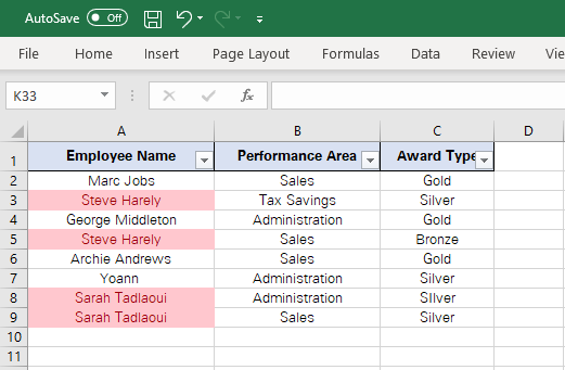
Excel is very well known and very widely used for data filtering. It facilitates many aspects of data cleaning and filtering that can help you save big on your time.

A common way of data filtering in Excel is eliminating duplicate data. And at times, removing duplicate data is not that simple. This is particularly the case when you want to delete rows that contain duplicate data in the same column.

But no worries! This article should enlighten you on three common and easy ways of filtering out duplicates from your data based on one column. Continue reading to learn them all.

1. The ‘Remove Duplicate’ Function

This is the easiest way to sweep your worksheets clear of duplicate values based on one column. Take a look at the data in the example below.

Award data for different employees

The above data represents the details of different awards won by employees in different areas.

Now, to filter out a distinct list of employees who won an award in any department, we need to filter duplicates from the column containing employee names i.e., Column A.

To do so, follow the steps given below.

Step 1:

Select the data to be filtered out along with the headers.

Step 2:

Go to Data Tab > Remove Duplicates as shown below.

Accessing the removing duplicates option from the Data Tab

This opens the ‘Remove Duplicates’ Dialogues box as follows.

The ‘Remove Duplicates’ Dialogues box

Step 3:

From the ‘Remove Duplicates’ Dialogues box, check the option ‘My data has headers’. This is because we selected the data including the headers.

Checking the option ‘My data has headers’

Step 4:

Unselect all the column headers appearing under the ‘Remove Duplicates’ Dialogues box. Only select the header for the column where the values to be filtered appear.

Unchecking all the columns except for one

Step 5:

Click ‘Ok’. Excel will remove the duplicate rows from the selected column.

Excel removes the duplicate rows from the selected column.

The results are as follows.

Duplicate rows deleted based on one column

Must note how Column A now only consists of a single instance for each employee name.

All duplicate or triplicate instances have been deleted from Column A and their corresponding entries from Columns B and C have also been deleted.

Pro Tip:
Unlike in this example, if you want to remove duplicates from more than one column, you can still use this method. The only difference to be made is of checking the boxes for other column heads.

2. Conditional Formatting

If you have a small dataset and you just don’t want to spend quite some time applying complex functions to your data, you can choose to go manual all the way.

An easy way to filter out duplicates based on one column is to conditionally format the duplicate values, filter them out, and delete them. Check out the example below.

Step 1:

Considering the same example as above. To identify the duplicates in Column A, select the said column and take the following route.

Home Tab > Styles > Conditional Formatting > Highlight Cells Rules > Duplicate Values

Accessing the conditional formatting rules

Step 2:

Set up conditional formatting options in the window that then opens up and click ‘Ok’. This would highlight the duplicate rows from Column A as follows.

Excel highlights the duplicate values from Column A

Step 3:

Filter out the highlighted values by applying data filters to your data as follows.

Select the header of Column A > Go to Data Tab > Sort & filter > Filter

Applying data filters to the data

Step 4:

This would add a drop-down menu icon to the header of Column A. Click on it and select ‘Filter by Color’.

Filtering out highlighted values

This would filter out highlighted values from Column A as shown below.

Highlighted values

From these rows, select duplicate rows and delete them to keep back only one row for each value.

Deleting duplicate values

Now remove filters and conditional formatting from your data to have the final look of your data without any duplicate values.

Data free of any duplicate values

3. Running a VBA Code

Both the above methods may seem easily accessible and convenient. However, if you have regular data-filtering to do, these methods may prove to be hectic and time-consuming. To counter the said problem, you may want to run a VBA Code.

You can set up a VBA code and add it to your Quick Access Toolbar to be able to readily access it only with a single click.

But you’re not a coder? No need to worry. You only need to copy-paste the following code, and you are done.

Sub Delete_duplicate_rows()

Dim Rng As Range

Set Rng = Selection

Rng.RemoveDuplicates Columns:=Array(1), Header:=xlYes

End Sub

Note: The above code is specifically built for the instance above, whereby in the code we have specified that the data contains headers and that data filtration is to be done based on Column 1 i.e. Column A. If you want to filter your data based on any other column, say column C, you may alter the second last line of the above code as Columns:=Array (3).

To run the code in your Excel, here are some easy steps to follow.

Step 1:

Go to the Developer tab from your Ribbon.

Pro Tip: If you find it nowhere on the ribbon, there’s nothing to fret about. 

Go to File > Options > Customize Ribbon > Check Developer’s Tab as shown below
Adding Developer’s tab to the Ribbon

Step 2:

From the developer’s tab, go to Visual Basic, and a VBA Window will launch as follows.

Launching a VBA Window

From the above VBA window, go to Insert > New Module. In the new module that opens up, write the code specified above and close the VBA window.

Writing the code into VBA

Step 3:

This creates a macro that is now ready to use. To access it, take the following route.

Developer tab > Macros

Accessing the Macros in Excel

From the list of Macros that then opens, select the ‘Delete_Duplicate_Rows’ macro and click Run. Excel would run the code, and the duplicates would be removed, as shown below.

Duplicate rows deleted by running the VBA Code

Pro Tip: Deleting duplicate rows by running a VBA code has no turn backs or undo options. Be very careful before you run this code and preferably keep a backup of your data to save yourself of any undue data loss.

Conclusion

Big Data is a common thing in the revolutionizing tech world. With more and more data coming in, we need more sophisticated and better techniques to sort and analyze data.

Filtering data of any duplicate values is one of those most-wanted techniques, and doing it in Excel can save you much time. The article talks about three ways how you can engineer your data in Excel – practice them all and learn them better.

Why a Dollar Sign is Used in Excel?

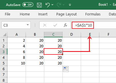
Have you ever seen ‘$’ in an excel sheet and wondered why is it so frequently used? To simplify things, ‘$’ means don’t change.

Sometimes, the $ in an excel sheet is just a dollar sign prefixing a currency value. Other times, it is used to lock a cell reference, often referred to as absolute referencing.

The article below covers all details on how and why a dollar sign is used in Excel.

What Means Dollar Sign in Excel?

A dollar sign in Excel comes in handy to prefix numbers (mostly currency) or to lock a cell for all changes of references.

It can be used as a simple currency symbol or for indicating absolute or mixed cell reference.

What that does is fix the value in a cell. With absolute reference, you lock the address of a cell.

However, with mixed cell reference, you have the option of locking any one of the two, the row or the column reference as per the needs.

A dollar sign is usually only used for indicating references in Excel. To understand what that means, let’s first learn about a cell reference.

What is a Cell Reference?

The address of a cell is referred to as cell reference. It tells Excel the location of the value that is to be put into the formula.

A cell reference is one of the most basic steps of learning Excel. First thing’s first – once you master the difference between references, you can master the rest of Excel in no time.

The formulas used can refer to multiple cells at one time and that makes Excel more powerful as the change of a single row or column can change the entire calculation.

Cell reference comes into use when a formula refers to a cell.

Here’s a quick example.

A cell reference in Excel

Whenever you select a cell in Excel, the ‘Name Box’ siding left to the formula bar displays the reference to that cell. In the above example, this turns out to be A2.

Note: The cell reference ‘A2’ is a combination of Column A and Row 2.

Alternatively, select any cell and add the operator ‘=’ to activate the cell for the formula. Click on any cell, and Excel would add the reference for that cell to the formula bar. Take a look below.

Cell reference in the formula bar

Let’s see the types of references in Excel and which one is related to the dollar sign as below.

Types of References

Excel offers three different types of cell references using which you can copy a formula to other cells. These are:

  • Relative references: The one that does not use the dollar sign at all.
  • Absolute references: The one that uses the dollar sign twice in a formula.
  • Mixed references: The one that uses the dollar sign only once.

Relative References

A relative reference is a cell address in Excel that changes with respect to the row and column number.

When you apply a relative reference to a cell and change its position, the reference changes according to the new position of rows and columns and adjusts to the new cell.

In excel, the relative reference is used by default.

Moreover, unlike other references, the dollar sign is not followed by the cell address in relative reference. In this way, the addresses can easily change, and each time you change the cell, you get a new result based on the given data.

Hence, a relative reference is a convenient method in Excel to deal with data when you want the references to be automatically adjusted for position changes.

It lets you perform the same calculation for corresponding cells across the whole worksheet. Let’s see an example below to visualize a better picture of how relative references work.

Setting up a relative reference in Excel

As seen in the above example, the formula ‘= A1 + 5’ when applied to cell B1, adds up the value of cell A1 and 5. If you now copy the formula to cell B2, the cell reference will change as in the following image.

Excel automatically updates the relative cell reference

The formula in cell B2 changes to ‘= A2 + 5’ unlike cell B1 as per the relative reference. Similarly, if we copy the formula to cell C1, the formula changes as ‘= B1 + 5’.

Change of reference in a new column

This illustrates how the relative reference changes for each cell when the same formula is copied at different places.

Also, for column B, simply try using the drag and drop function and see how Excel updates the cell references for every single cell in a snap.

Absolute References 

An absolute reference is the cell address that uses two ‘$’ signs in one formula. One lets you lock the row and the other, the column.

When this reference is used, the cell reference remains the same no matter which cell of the worksheet it is copied to.

To use absolute reference for a cell, it needs to be applied manually to the cell in question.

Unlike relative reference, both the row and column names are preceded by dollar signs.

This is mostly used when you have large sets of data, and you must apply the same formula to all cells in a worksheet. So even if you change the position of the formulas, you will still have the absolute cell references unchanged.

Let’s see an example below to understand the concept better.

The absolute reference remains the same in B1

As visible, the absolute reference formula applied to B1 remains the same and will give the same result no matter which cell you copy it to.

Constant cell address for all locations

The formula in cell C3 remains the same as in B1 because of the absolute reference.

There are only a handful of instances where you use absolute references independently in a worksheet. This is because most of the time, absolute and relative references are both used together.

Pro Tip: If you do want to change the absolute reference, add a row or column. Although absolute reference locks the cells and does not move from the origin, on the addition of a new row or column, it leaves the previous location and adjusts with the new row or column.
Setting up the formula =$A$1*10 in Cell B1

In the above image, the formula in cell B1 is =$A$1*10.

Adding a new column to Excel

Upon adding a new column, the values shifted to the next column, and the cell reference in cell C1 became =$B$1*10.

Mixed References

A mixed cell reference is super simple and easy to use.

Unlike absolute reference, mixed reference locks only one coordinate, i.e., it uses only one dollar sign – either before the column name as $A1 or before the row number as A$1.

In $A1, the column name is locked and will not change but the row number can be adjusted. Similarly, in A$1, the column name can be adjusted but the row number won’t change as it is fixed.

Let’s see the image below to grasp the concept better.

=$A2*$B2+C$2

Mixed cell references applied to the formula

As seen in the image above, cell C3 contains mixed cell references. In the first two cell references, the column name is locked and in the third cell reference, the row is locked.

When you put $A2 in the formula, Excel will change the row number orderly, but the column name will remain the same.

Similarly, in $B2, the column remains the same, but the rows change for each cell where the formula is copied.

In C$2, the row will remain the same, but the three instances in three different columns will be used sequentially.

Shortcut to Add Dollar Sign

Adding or removing a dollar sign is easy. You can either do it manually or use a shortcut key to perform the task.

If you want to manually add a dollar sign, simply double-click on the cell to activate it (or press the F2 key). Place the cursor where you want to add the dollar sign and hit the dollar key.

Usually, when the shortcut is used, it adds or removes the dollar sign for references. The shortcut key used is F4. Single-click on the cell which contains the formula and press the F4 key. The key will let you toggle among the following four instances:  

  • Upon pressing the F4 key once, a dollar sign is added to the cell reference.
Pressing the F4 key once

  • Upon pressing it the second time, another dollar sign is added.
Pressing the F4 key twice

  • Upon pressing it the third time, a dollar sign is removed.
Pressing the F4 key thrice

  • Upon pressing it the fourth time, another dollar sign is removed.
Pressing the F4 key four times

In this way, you can activate relative, absolute, or mixed references as needed. Or, you can remove dollar sign to turn your cell reference from absolute to mixed to relative reference.

Pro Tip: Make sure to activate the cell, or else, upon pressing F4, Excel will automatically select the cell to the left of the cursor and change its reference type.

Conclusion

A dollar sign has much more uses in Excel than being prefixed to a number for representing currency. You may use it to turn cell references into absolute cell references or mixed references with sheer ease.

Practice a few examples stipulated above to master using the $ sign in Excel in no time. Happy Excel Exploring!