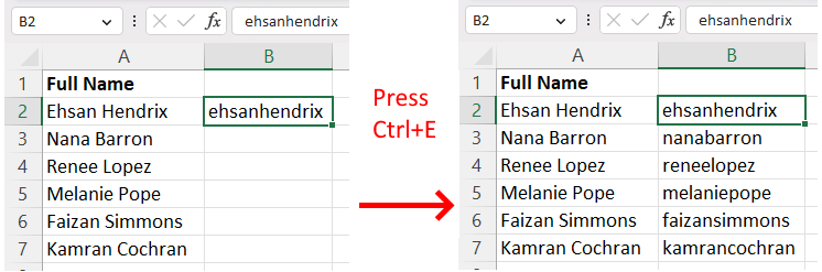
Excel has many useful functions and tools that enable us to perform text manipulation. That’s why, when you have first and last names in separate columns in a spreadsheet, it’s extremely easy to combine them into a full name, whether you want it separated with a space or a comma.
In this tutorial, we will learn how to combine first and last names in Excel using the CONCATENATE function, the ampersand (&) operator, and Flash Fill.
Table of Contents
Using the CONCATENATE Function to Combine First and Last Name
The CONCATENATE function enables us to combine multiple cells or values. We can use this function to combine first and last names and separate them with a space or a comma. Let’s learn how…
Write the following formula in a new cell to combine first and last names with a space:
=CONCATENATE(A2, " ", B2)
The first cell name (A2) refers to the first name, and then we concatenate the space character (“ “), and the last name (B2).
You can drag the small green rectangle in the bottom right of the cell with the formula, and drag it downward to apply the concatenate operation to other cells.
If you want to combine the names with a comma with the format “LastName, FirstName”, use the following formula:
=CONCATENATE(B2, ", ", A2)
The CONCATENATE function can combine multiple text values or cells. Therefore, it can also be used to combine a first name, middle name, and last name:
=CONCATENATE(A2, " ", B2, " ", C2)
So, the trick is: to write all the cell values and separators inside the CONCATENATE formula and separate them with commas. When you learn this simple formula, you can combine anything!
Using the Ampersand (&) Operator Function to Combine First and Last Name
Text combination can also be achieved with the ampersand (&) operator. Write the following formula to combine first and last names with a space:
=A2&" "&B2
If you want to combine the names with a comma, type the following formula in a new cell:
=B2&", "&A2
The ampersand operator (&) works as follows: you need to start the formula with the equal (=) sign, and then write the cell names and separators, and type ampersand (&) between each of them. This is another elegant way of combining first and last names.
Using Flash Fill to Combine First and Last Name
Without using operators and formulas, it is perfectly possible to combine first and last names: with the help of Flash Fill. Flash Fill is a tool that learns and applies patterns. Follow the steps below to combine using Flash Fill.
Step 1: Next to the first and last names, write the full name in a new cell.
Step 2: Go to the cell below by pressing Enter, or clicking on the cell.
Step 3: In the Home tab, click on the Fill icon in the Excel ribbon, and then click on Flash Fill.
Flash Fill will automatically learn the pattern, and combine the first and last name for all cells.
You can apply the same steps if there are middle names in your data. As long as you type the full name exactly as in the original cells that contain the first, middle, and last names, the combination pattern will be learned and applied by Flash Fill.
In this tutorial, we learned how to combine first and last names in Excel using the CONCATENATE function, the ampersand (&) operator, and Flash Fill. You can choose whichever method suits you best.
A cumulative percentage is a statistical tool commonly used in analyzing scientific research, finance, and sales data. But what exactly is it, and what is its purpose?
Table of Contents
Cumulative Percentage is defined as a way of expressing frequency distribution. It shows the percentage of the cumulative frequency within each interval.
Essentially, it can be viewed as the percentage of the accumulated total over time (or over certain intervals).
It can be used to understand how much progress has been made over time.
If you look at the image below, the first two columns show the total sales for each month. The third column is the Cumulative Frequency (or the running total). The fourth column shows the Cumulative Percentage (or the percentage of the accumulated totals).
Looking at this table can already give us an idea of how much progress has been made by this pseudo business over time.
When it started in January, it only earned 5% of what it is making today (December).
After 6 months (or in June), it earned more than half (52%) of the overall total.
As you may have noticed, the Cumulative Percentage gives us a better visual representation of the growth (as compared to the Cumulative Frequency).
Please know that Cumulative Percentage is not only limited to date intervals.
If you look at the table below, the first two columns show the number of students that earned a particular exam score. The last two columns show the Cumulative Frequency and Percentage.
Looking at this table, we can conclude that 72% of the students only got a score of 70 and below, which could mean that 72% of them didn’t pass (if 80 is the passing score).
As you can see, cumulative percentages can be used in varying datasets and can be interpreted in many ways.
Now, I’ll show you how you can calculate the cumulative percentage of your data in Excel.
1. Using Formulas to Calculate Cumulative Percentage
1. Set up your dataset. Add the interval on the 1st column and the value on the 2nd column.
Remember to sort the records in the correct order. It should be sorted from oldest to newest if it’s a date interval.
2. Now, we’ll add the formulas of the Cumulative Frequency in the 3rd column.
On the first cell, write this formula: =B2
Note that it should point to the first value in the dataset.
On the second cell, write this formula: =B3+C2
This formula sums up the current amount and the cumulative frequency of the previous row.
Next, copy this formula to the remaining rows in the column using the Fill Handle.
Click on the cell with the formula and hover your mouse on the right side of the cell until the Fill Handle appears (or until the mouse cursor turns into a black plus sign [+]).
Once you see it, drag your mouse down until you reach the last row in your data set.
You should now see your Cumulative Frequency column all filled out.
The last cell in this column is the overall accumulated total since the start of the dataset.
We will use this cell to calculate the Cumulative Percentage.
3. On the fourth column, write this formula: =C2/$C$13
Change $C$13 with the last cell in your Cumulative Frequency. Remember to add anchors or dollar sign ($) in the cell reference so that it always points to this cell.
This formula divides the CurrentCumulative Frequency with the LastCumulative Frequency to get the percentage value.
Once you’ve added the formula, copy it to the remaining cells in the column by dragging the Fill Handle down.
4. As the final step, convert these cells into percentage format.
Select all the numbers in this column. Go to the Home tab and click on the percentage button inside the Number section.
And that’s it! You now have your Cumulative Percentage calculated.
Note that the last cell in the column should be 100%, reflecting the percentage of the highest accumulated value.
2. Using Pivot Table to Calculate Cumulative Percentage
Using Excel’s Pivot Table is probably the quickest way to get the cumulative percentage.
1. Select your entire dataset.
Note that your dataset should be sorted in the correct order.
2. From the Insert tab, click on the Pivot Table button.
3. The “PivotTable from table or range” menu will appear.
Select where you intend to add the pivot table – whether on a new worksheet or a specific range in the current worksheet – then click OK to continue.
4. The PivotTable Field List will appear on the right.
Drag each field to its corresponding areas in the pivot table.
The interval should be in the Rows area, and the value should be in the Values area.
By default, the Pivot Table will get the sum of the value field.
We will change it so that it displays the Cumulative Percentage instead.
5. Right-click on any cell containing the value field in the Pivot Table and select Value Field Settings.
6. The Value Field Settings menu will appear.
Change the Custom Name with the appropriate name for the field. You can name it “Cumulative Percentage”.
Go to the Show Values As tab.
In the “Show values as” dropdown menu, select %Running Total In.
In the “Base field”, select the interval.
Once done, click OK.
And that’s it! You now have your cumulative percentage calculated!
What’s great with this method is that if you have new rows added to your dataset, you only need to update the pivot table’s data source and you’re good to go!
Conclusion
Cumulative Percentage has various uses in different industries. No matter what your purpose for it is, I hope this tutorial helps you easily calculate it in Excel. Whichever of the two methods you choose, please remember to always sort your dataset in the correct order before adding the formulas or the pivot table.
An IF statement is a function in Excel that enables us to determine whether a particular condition is met.
For every condition, there are only two possible answers:
TRUE, if the condition is met
FALSE, if the condition is not met
It uses the following syntax: =IF(logical_test, [value_if_true], [value_if_false])
logical_test
Refers to any value or expression that results in either TRUE or FALSE.
We usually use logical operators in this argument to compare values (see table below for reference).
LOGICAL OPERATOR
MEANING
=
Equal to
<>
Not equal to
>
Greater than
<
Less than
>=
Greater than or equal to
<=
Less than or equal to
value_if_true
Refers to the value returned if the logical_test is true.
If omitted, the word TRUE becomes the returning value.
value_if_false
Refers to the value returned if the logical_test is false.
If omitted, the word FALSE becomes the returning value.
When working with an IF statement, we can think of it as a flowchart with two pathways – one is for TRUE, and the other is for FALSE.
There are instances, however, when we need to evaluate more than one condition before displaying a value. It’s when the multiple IF statements come in.
We can add the additional IF statement in either the value_if_true or the value_if_false argument. We can even add it on both — turning the flowchart to look something like this:
As you can see, the flowchart has significantly increased in size with just a few IF statements inserted.
It gets even more overwhelming when you look at multiple IF statements from the formula bar in Excel (see example below).
Excel allows up to seven IF functions nested or joined together, but that doesn’t mean you should use all of them.
Multiple IF statements, if improperly curated, can be a source of frustration when fixing issues related to them. It takes a lot of thought to build them and even more to update and debug them.
As much as possible, make it a rule to simplify your formula and take advantage of other available Excel functions to perform the logical comparisons. You could, for example, use VLOOKUP instead of nested IF statements. This way, you won’t have a very lengthy formula to maintain.
Don’t worry. I’ll provide some suggestions below to help you write a shorter formula that still fulfills the requirement of conducting multiple logical tests before displaying a result.
Table of Contents
How to write a multiple IF statement in a cell in Excel
Before writing a multiple IF statement in a cell, create a table containing the conditions and the corresponding results that you want to add to the IF statement.
This table can help you arrange the conditions accordingly. When writing multiple IF statements, remember that the order of the conditions (or the logical tests) matters significantly.
Once the initial logical test is met, Excel no longer goes through the remaining conditions or tests.
In the screenshot below, notice that I have two tables added.
The table on the left shows a list of students with their grade percentages. In column C, I intend to add a formula that gets the corresponding Grade Letter based on the Percentage.
The table on the right shows a list of all the Grade Letters with the corresponding Percentage. These are the set of conditions that I will use for the IF statements.
Now, I’ll start adding the first condition: =IF(B2>=90, “A”
This line says that if cell B2 is greater than or equal to 90, the grade letter is A.
Next, I’ll add the second condition (another IF statement) in the value_if_false argument. The formula will now look something like this:
Keep adding the conditions (the IF statements) in the value_if_false argument until you have added the last one.
The last step is to specify the value to display if all the conditions are unmet. In my case, I added a blank value (“”).
After adding all the conditions, add all the closing parentheses for each IF statement.
That’s it! You have your multiple IF statements all set. If set up correctly, you should be able to generate the correct output.
IFS function: An alternative function
Working on a formula with multiple IF statements can be a handful. You will see lots of “IFs” and parentheses (). Updating it can be confusing and overwhelming at times.
Excel offers an alternative to this, that is, the IFS() function.
IMPORTANT NOTE:
The IFS() function only works on Office 2019 and Office 365.
Unfortunately, this feature is not available on other versions.
The IFS() statement has a pretty straightforward syntax:
It starts with a condition followed by the value to display if the expression returns true.
If you want to add another condition, add a comma and proceed with adding the expression and the corresponding result. And so forth.
Pretty simple, right?
The image above shows the difference between a multiple IF Statement and an IFS statement.
Note that the IFS statement is much shorter. The word “IF” and the parentheses no longer appear more than once, making it easier to read and update.
You must remember that just like the multiple IF statement, the order of the conditions matters in an IFS statement. Once the first condition is met, Excel no longer evaluates the remaining conditions.
Excel allows up to 127 conditions in the IFS statement. But, as mentioned, I don’t recommend you use all of it. Make it a point to simplify your formulas. That will save you from unnecessary headaches in the long run.
VLOOKUP function: Another alternative function
A terrific substitute for the nested IFS is the VLOOKUP function. If your conditions are also based on matching the numbers within a particular range, VLOOKUP is for you.
The VLOOKUP function enables you to find an item from a table. What’s cool about this function is that you have the option to configure how the lookup is performed. It could be by “exact match” or “approximate match”.
In the “Search for Grade Letter” example, it would be more appropriate to use the approximate match method. This option tells Excel to find the closest value in the table.
For it to work, the first column in the reference table (the one that will be used for matching) should be sorted in ascending order (with the smallest number on top).
To do this, let’s start by converting the reference table to something similar to the image below:
1. Get the lowest percentage value and place that on the first column of the table. In your case, this would be the lowest number in the range.
2. In the next column, add the Grade Letter (or in your case, the result that you want to appear if it matches the first column).
3. After that, sort the first column so that it’s in ascending order.
That’s it! Your reference table is now all set. The final step is to add the VLOOKUP formula.
Refers to the value to search for in the first column of the reference table.
It can either be a value or a range.
table_array
Refers to the range containing the reference table.
col_index_num
Refers to the column number in the table_array that contains the value to be returned if a match is found.
Note that the first column of values in the table is column 1.
[range_lookup]
Set to TRUE to find the closest match in the first column.
Set to FALSE to find the exact match in the first column.
In the screenshot below, see how significantly short the formula has become compared to when I used the multiple IF statement.
What’s also great about VLOOKUP is that it eliminates the need for you to update the formula to add more conditions or edit the existing ones.
You only need to update the reference table, and you’re all set! Any changes in the conditions and resulting values will immediately take effect.
Conclusion
Multiple IF statements in a cell are OK if you are working with a limited number of conditions. As mentioned, it can be quite taxing to build and maintain. So, give the others (or your future self) a favor and simplify the formula as much as possible. You may also want to explore other Excel formulas that you could use (e.g., IFS, VLOOKUP).
We frequently use Excel to calculate different kinds of averages (mean, median, mode etc.) for different sets of numbers. The size of the dataset varies and can often be super huge.
The contemporary mean function finds the average of a data set by adding up all the values of the dataset and dividing them by the number of values. However, mean is often only calculated for a sample of the population and not for the entire population.
This can lead to errors. And to counter these errors caused by computing the mean for only a sample from the population, we estimate the standard error.
Table of Contents
What is a Standard Error?
The standard error of mean is used to estimate the difference between the mean of a sample and the true mean of the entire population. Must’ve made only a little sense. See below.
An Example:
Suppose you take up the project to estimate the average age of the people of a town that has a population of 1 million. It might not be feasible for you to collect data for every single person from this population. So, you may resort to sampling by picking up a sample size of 5000 people out of the total population.
Noting down the age of each of these 5000 people, you can find the average age for this sample. This can then be projected to the entire population of 1 million. Let’s say, this number works out to be 32 years.
The average age of 32 years is an approximation of the average age for the people living in that town. However, as this average age is only computed based on a sample, there are high chances that it won’t be a true representative of the entire 1 million population.
Had you averaged out the age of all the 1 million people living in that town, the results might have been slightly different – say 32.7 years.
This error of 0.7 (32.7 less 32) is a standard error.
Note: A standard error is negatively correlated to the sample size. The larger the sample size, the smaller the standard error.
How To Calculate Standard Error?
A standard error is the approximate standard deviation for a given sample. Excel doesn’t offer an in-built function to calculate the standard error for a given dataset in one go. However, by combining a few functions, the standard error for a given dataset can be conveniently found in Excel.
There are two ways how this might be calculated in Excel. Let’s look into them both.
1. A mathematical formula
The formula below must take you back to your school times.
Not only relevant theoretically, but you can also apply this formula to Excel by breaking down the calculation into a few simple steps.
In the image below, we have a data set that has 10 numbers.
To find the standard error for the mean of these 10 numbers using the above formula, stick to the steps below.
Step 1:
Calculate the average for the sample data using the AVERAGE function of Excel as shown below.
Step 2:
Calculate the difference for each value from the dataset against the average for the data set.
Pro Tip: If you plan on using the ‘Drag and drop’ function of Excel to calculate the differences in a snap, do not forget to turn the cell reference containing the average into an absolute reference. To do so, simply click on the cell reference in the formula bar (B14 in this case) and press F4.
Step 3:
Square the differences (Column B).
Pro Tip: If the exponential power sign (^) is nowhere to be found on your keyboard, do not worry. You can set up the formula as (B2 * B2) or (B3 * B3) etc.
Step 4:
Sum up the square values.
Step 5:
To take the formula ahead, you need to know the number of data points, which in the given example is 10. In the instance under question, the count was an easy one and could have been performed manually.
However, this might not always be possible, particularly with voluminous data sets. To find the number of data points, you can employ the COUNT function as follows.
= COUNT ( A2: A11 )
Step 6:
While we have all our figures ready, it’s time we put them into the formula to find the Standard Error as shown below.
= SQRT (B15 / (B16 * (B16-1) ) )
And there you have the standard error of 0.5617, all calculated in Excel.
2. Combining the STDEV.S and SQRT function
Another method how you may find standard errors in Excel is by using the standard deviation and the square root functions of Excel.
A short way to compose the mathematical formula explained above is as follows.
In the above formula, the sign ‘σ’ represents ‘standard deviation’.
Simply put, standard error can be calculated by dividing the standard deviation for a given dataset by the square root of the number of data points in a dataset.
The example below should demonstrate how this formula can be applied in Excel.
Step 1:
Continuing the same data set as above, the first step is to calculate the standard deviation for the dataset. Excel offers an in-built function to calculate standard deviation and all you need to do is set up the formula.
= STDEV.S (A2:A11)
Step 2:
Calculate the number of data points in your dataset, you may want to do this manually or by using the COUNT function.
= COUNT ( A2: A11 )
Step 3:
Put together the formula for standard error by using the SQRT function as demonstrated below.
= B14 / SQRT (B15)
Excel calculates the standard error of 0.5617.
Must note how the answer remains constant between both the methods of computing standard error in Excel.
How To Put Standard Error Bars In Excel?
For a better visual representation, you can turn your dataset into a graph. For instance, in the image below, three bars represent three different averages.
After a bar chart has been constructed, you may add standard error bars to it to know the possible deviation in actual results. To add standard error bars to your bar chart, follow the steps below.
Step 1:
Click anywhere on the chart to activate the chart formatting options. Tap on the ‘plus’ sign on the right and choose ‘Error bars’ as shown below.
Step 2:
This will add error bars to the top of each bar, as shown above. Click on these small bars to open editing options for the same.
From these options, select ‘Standard Error’ and other options to shape the error bars as you may like.
Adding error bars to Excel is only that easy, and this helps the viewers know the possible extent of deviation from the visualized figures.
Conclusion:
Mean and other averages are super common and massively used in all fields of life – be it a mathematics assignment or a statistical forecasting model. With such extensive use of sample averaging methods, it is essential to know the possible loopholes with sample averaging.
Not only that, but you must also know and master measures to counter the effects of such loopholes. Calculating and adjusting the standard error is one of them, and with Excel, this calculation becomes super easy.
Practice with the examples stipulated above to master standard error calculation.
To find the average of only those values that meet a specific criterion, you need to employ the AVERAGEIF function in Excel.
Learn all about this function in the article that follows.
Table of Contents
AVERAGEIF Function
The AVERAGEIF function of Excel is a statistical function that allows users to average only those cell values that meet a specified criterion. The specified criteria can include text, logical operators like >, <, =, < > and wildcard characters too.
Syntax
Syntax of the AVERAGEIF function is stated as follows.
= AVERAGEIF (range, criteria, average_range)
Arguments
Let’s break down the above syntax to see how each of its arguments function.
Range – The criterion specified for averaging specific values is looked up from this range. This can be a single or more cell, any reference, or value.
Criteria – This includes the criterion based on which specific values are to be averaged.
Average_range – This defines the range containing values that are to be averaged. If left vacant, Excel automatically assumes this argument equal to the range (first argument).
Return Value
The AVERAGEIF returns the average of those values from the range that meet the specified criterion.
Functions Library
You may access the AVERAGEIF function from the Functions Library in Excel as follows.
It’s time to delve into some examples to learn how the AVERAGEIF function practically works and how can you use it to your benefit.
1. Simple operation of the AVERAGEIF function
Below is a screenshot that manifests sales of different regions for different years.
To find the average sales in Toronto over the given years, here’s what needs to be done.
Step 1:
Activate the cell where you want the average value to be populated and compose the AVERAGEIF function as follows.
= AVERAGEIF (C2:C11, “Toronto”, “B2:B11”)
The range is defined as C2:C11, where the criterion is to be looked up for as this column contains the region information.
The criterion i.e. Toronto is enclosed in double quotation marks “Toronto”. This is because it is a text value.
The average_range is specified as B2:B11, where the values to be averaged are populated.
Step 2:
Hit enter to see the following results.
Excel has calculated the average of all those sales whereby the corresponding region is Toronto.
2. Using AVERAGEIF function with logical operators
Sometimes the criteria that you specify is not only a single value but a condition. For example, average all numbers greater than 3, etc.
You can apply the AVERAGEIF function to find similar averages by employing logical operators. For a quick reiteration, logical operators that can be used in Excel are as follows.
Logical Operator
Meaning
=
Equal Sign
>
Greater than
<
Less than
<>
Not equal to
>=
Greater than or equal to
<=
Lesser than or equal to
An example can help us learn better how logical operators may be used in pair with the AVERAGEIF function.
Step 1:
Continuing the same example, as above, if we want to calculate all those sales that are equal to or greater than $5000, compose the AVERAGEIF function as follows.
= AVERAGEIF (B2:B12, “>=5000”)
The range is set as B2:B12 as the values are to be looked up are populated under column B.
The criterion is set to “>=5000”. The Logical operator >= signifies greater than or equal to 5000. It is important to enclose the criterion in double quotation marks for Excel to recognize it as text.
We want Excel to calculate the average of sales based on a specific sale value. As the range and average_range in the foregoing example are the same, the last argument can be omitted. Excel will assume the average_range to be the range.
Step 2:
Once the formula is devised, hit enter to see the following results.
Excel has calculated the average of all those sales that are equal to or greater than $5000.
3. Using AVERAGEIF function with wildcard characters
Wildcard characters and their appropriate usage can help you straighten out many things you thought you’d keep laboring about.
Wildcard Characters
Usage
*
Equates to any number of characters in any order
?
Equates to any single character in the same order
Take a look at the example below to better decipher the application of wildcard characters.
The image below represents Sales made to different customers.
A deeper look into the data tells that in many instances, the name of the same customer is spelled differently. For example, Sania can be seen spelled as, Sanea, and Sanya, when she is the same customer.
If we want to find the average sales per customer, how can we define a criterion that meets all these spelling variants?
Step 1:
Wildcard characters can be used to do so. Compose the average formula as follows.
= AVERAGEIF (A2:A11, “San?a”, B2:B11)
The range is set to A2:A11, where the customer name is to be looked up for.
The criterion is set to “San?a” as all the three spelling variants involve a different 4th letter. Substituting the fourth letter with a wildcard character (?), Excel would consider all spelling variants irrespective of the fourth character.
The average_range is set to B2:B11 where the sales are populated.
Step 2:
Hit enter to see the following results.
Excel has calculated the average of cells containing all spellings of Sania with a varying fourth character.
Troubleshooting the AVERAGEIF Function
The AVERAGEIF function is one of the most basic functions of Excel and is likely not to trouble you unduly. However, keeping in mind the following pointers can help you get rid of any problems that users commonly encounter with the AVERAGEIF function.
Empty Cells – The AVERAGEIF function ignores those cells that are vacant. These cells are not included in the computation of average.
#DIV/0! Error – Excel will give back the #DIV/0! Error when none of the cells meet the criteria specified by you. This technically means that no value is to be averaged.
Range Compatibility – The argument ‘range’ and ‘average_range’ in Excel necessarily need not be the same in size.
Conclusion:
The AVERAGEIF function can help you get through so many of your routine tasks in Excel. A little practice of the said function can help you master the same.