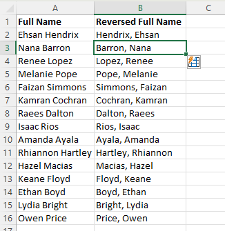
How to Switch First and Last Name in Excel
Data manipulation is one of the most powerful abilities of Excel. Flash Fill is a tool in Excel that enables you to manipulate data in a cell according to your needs. In this tutorial, we … Read more
Check out a wide range of Excel topics, from basic functions and formulas to more advanced topics like VBA and macros.
Data manipulation is one of the most powerful abilities of Excel. Flash Fill is a tool in Excel that enables you to manipulate data in a cell according to your needs. In this tutorial, we … Read more
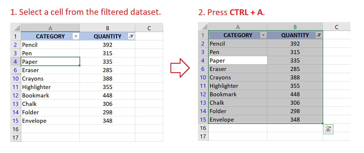
Copying filtered data onto a new sheet is a great way to segregate related data rows. It allows us to have the extracted rows available anytime without re-applying the same filters. We have to be … Read more
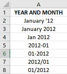
When working with exported data, there will be times when we will have only the month and year included in the dataset (the day is nonexistent). It was okay until you realized that, for very … Read more
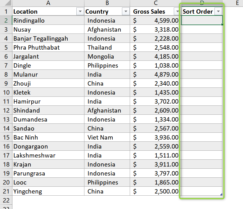
Data sorting (or the process of arranging data based on a field or a set of fields) allows us to analyze data more effectively. If you want to temporarily sort your data in a particular … Read more
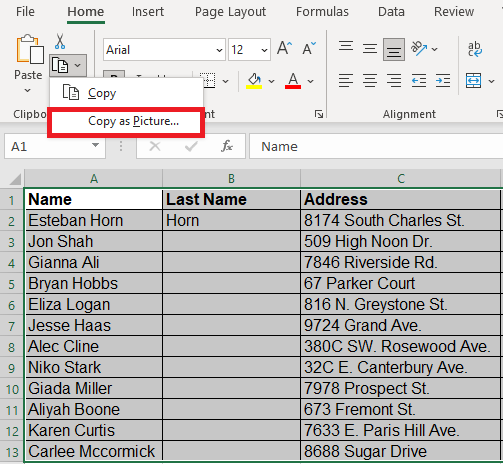
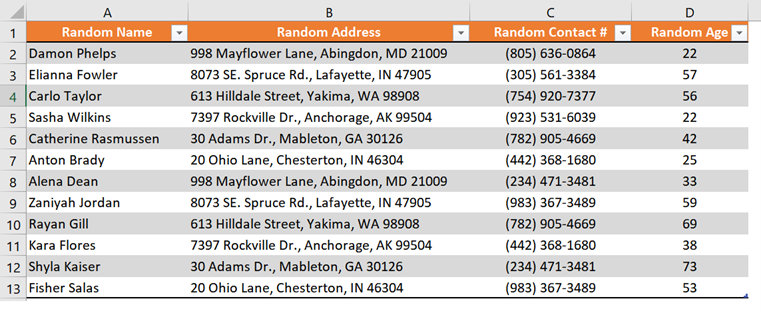
Excel is a great way to store, compute, and sort information; however, there may be times when you want to save the tables in Excel as images for use on the web, brand print material, … Read more
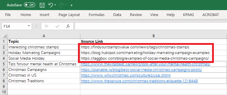
Have you ever imported data to Excel from an external source with many unwanted hyperlinks that came along? Also, you might have come across multiple undesired hyperlinks automatically generated by Excel for emails and URLs … Read more
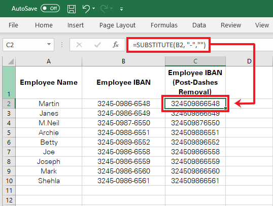
If you’ve ever worked in an HR role, you know how challenging it can be to maintain a large volume of personal details for multiple employees, including their CNIC numbers, IBANs, Passport numbers, or even … Read more
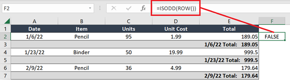
Data exported from a system are usually in a fixed report format. Sometimes though, it even includes unnecessary rows in between the data. In my example below, notice that there’s a total row added between … Read more
Adding alternate row colors in your data is a great way to enhance its readability. It makes it easier for your intended audience to find a record and see its related information. Plus, it’s so … Read more
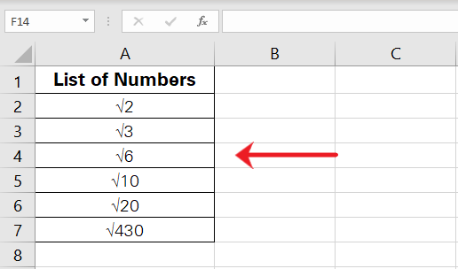
Before anything, what is a square root symbol? Let me quickly take you back to high school mathematics. Here’s what the square root symbol looks like. We often need this symbol in your spreadsheets for … Read more