If you have worked on a large dataset before, you would know the importance of always having the field headers visible even as you scroll through the sheet to go over the rest of the data.
It saves us a ton of time from scrolling back on top or to the left just to remember what field we are looking at.
In this article, I will show you ways to keep a particular area in your worksheet “locked” or “frozen” even as you move to a different section in your sheet.
How to Freeze the Top Row in Excel?
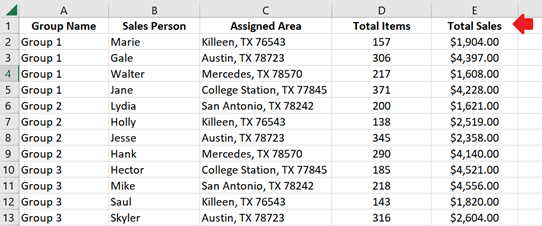
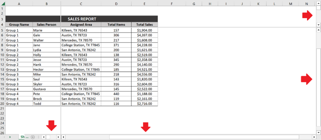
Datasets in a typical format usually have the headers in the first row of the worksheet (as shown in the image below).
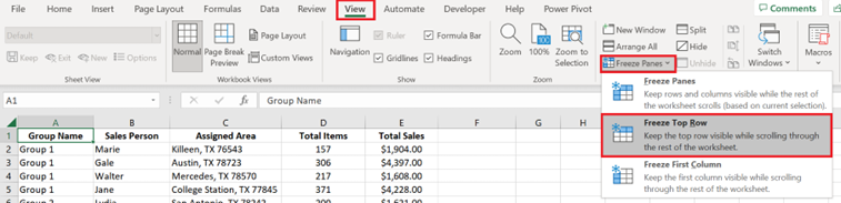
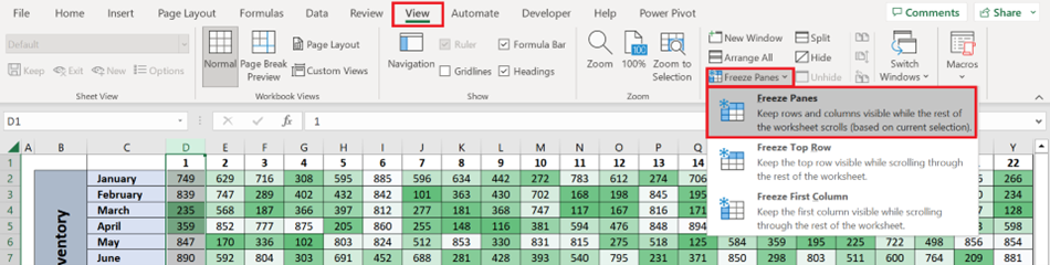
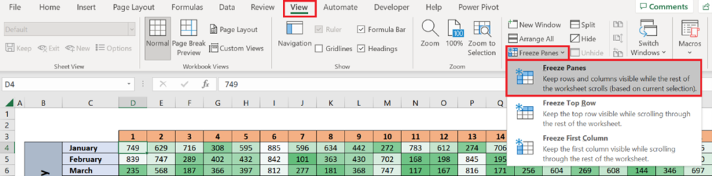
To freeze the top row of a sheet, go to the View tab.
From the Window section, click Freeze Panes and select Freeze Top Row.
And that’s it! The top row is locked on top even as you scroll down.
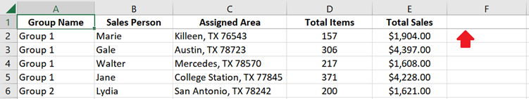
The gray horizontal line serves as a marker indicating that the row on top of it is frozen.
How to Freeze Multiple Rows in Excel?
If you want to freeze more rows (other than the first row), you only need to:
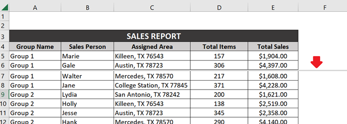
1. Select the entire row just below the rows you intend to freeze.
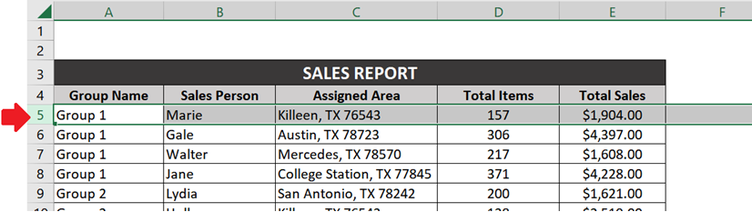
In my example above, I wanted to freeze rows 1 to 4, so I selected row #5.
2. Once the entire row is selected, go to the View tab.
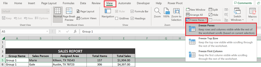
From the Window section, click Freeze Panes.
From the list of options that appear, select Freeze Panes.
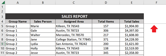
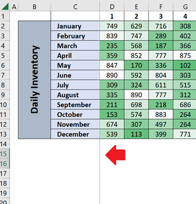
3. And that’s it! The rows above the selected row are now frozen.
How to Freeze the First Column in Excel?
To freeze the first column in your worksheet, go to the View tab.
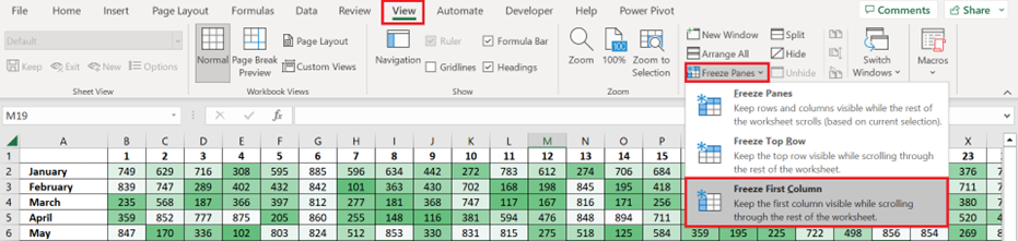
From the Window section, click Freeze Panes and select Freeze First Column.
And that’s it! The first column in your sheet is now locked and will no longer move even as you scroll to the right.
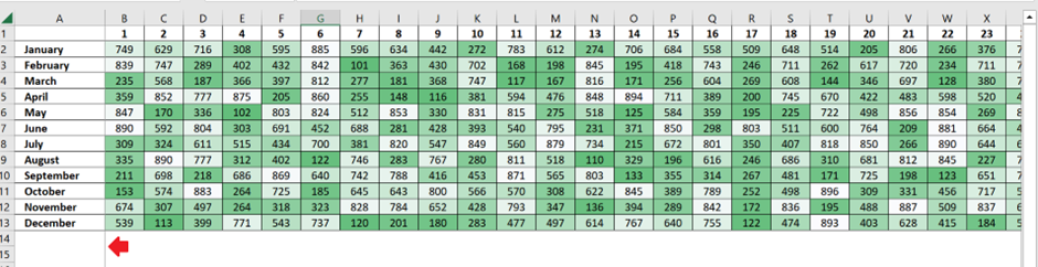
The gray vertical line serves as an indicator that the column before it is frozen.
How to Freeze Multiple Columns?
If you want to freeze more columns (other than the first one), you only need to:
1. Select the entire column that comes after the columns you intend to freeze.
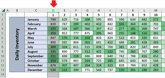
In my example above, I wanted to freeze columns A, B, and C, so I selected column D.
2. Once you have selected the entire column, go to the View tab.
From the Window section, click Freeze Panes and select Freeze Panes from the list of options.
3. And that’s it! The columns before the selected column are now “locked” even as you scroll to the right.
How to Freeze Both the Rows and Columns in Excel?
If you have headers on both the top and left sides of your dataset, you will need to freeze both rows and columns. To do this:
1. Find the intersection between the top rows and the left columns that you intend to freeze.
2. Then, select the cell just after that intersection.
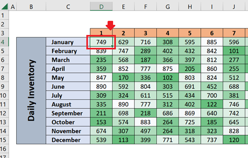
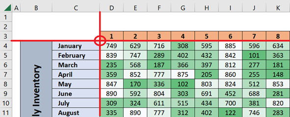
In my example above, I wanted to freeze rows 1 to 3 and columns A to C, so I selected cell D4.
3. Once the cell is selected, go to the View tab.
From the Window section, click Freeze Panes and select Freeze Panes from the list of options that pop up.
4. And that’s it! You now have your top rows and left columns locked and frozen even as you scroll up and down.
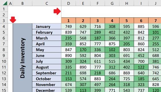
The gray horizontal and vertical lines serve as a marker to indicate which rows and columns are frozen.
INSIGHT:
As you may have noticed, we can only freeze the rows on top and the columns on the left. We cannot do it with the rows at the bottom and the columns on the right.
Freezing Panes is both top and left-oriented. Therefore, if you wish to keep a particular set of cells always visible, you will need to place them on the rows at the top or on the columns at the left.
How to Unfreeze the Rows and Columns in Excel?
To unfreeze the rows and columns, you only need to:
- Go to the View tab.
- From the Window section, click Freeze Panes and select Unfreeze Panes from the list of options that appear.
- You’ll know that the panes are no longer frozen once the gray horizontal and vertical lines disappear.
Why are the “Freeze Panes” Buttons in Excel Disabled?
There are three possible reasons why the “Freeze Panes” buttons in your View tab are disabled:
- You are in the middle of editing the content of a cell (e.g., typing a formula in the formula bar). Solution: Finish writing the formula and press Enter (or press ESC to discontinue the changes you are working on).
- Your worksheet is protected. Solution: Unprotect the worksheet first.
- You are in the Page Layout view. Solution: Switch the view to Normal.
Alternative to Freezing Panes in Excel: Split Panes
“Split Panes” is a considerable alternative to freezing panes if you intend to compare records against each other. With this method, you can keep a particular set of rows or columns visible as you scroll through the sheet.
The steps in splitting panes and freezing panes are pretty much the same.
- If you want to split some rows, select the entire row that follows after them.
- If you want to split some columns, select the entire column that follows after them.
- If you want to split some rows and columns, select the cell where the rows and columns intersect.
Once the appropriate row, column, or cell is selected, go to the View tab.

From the Window section, click on Split.
A thick gray line will appear on the sheet. This line indicates where the rows or columns split.
Notice also that there is one scroll bar added for each pane.
You can use these scrollbars to move to a different area for each pane.
Please remember that this method is not the same as “freezing the rows or columns” per se. It is only giving us a split view of the cells. So, if you happen to scroll through each pane and move to the same area, your worksheet can look something like this:
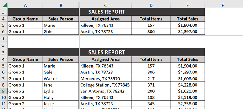
Both panes now have the same contents.
Conclusion
As you can see, freezing the top rows or left columns can be done in just a few clicks. If you are freezing more than one row or column, you only need to pay attention to which cell (or row or column) you need to select before freezing the panes. I hope this article helps!