Have you ever worked on a set of data with blank rows in between? It can be pretty annoying, right?
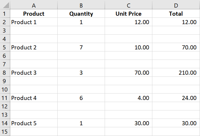
Table of Contents
Oftentimes, we do encounter this format of data whenever we export data from a system or a database.
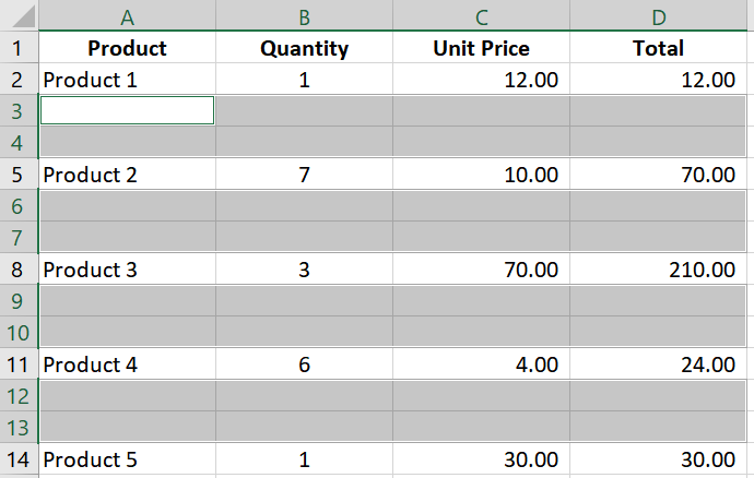
With the blank rows in between, it’s quite difficult to sift through the data as you have to scroll further down just to see the rest of the records.
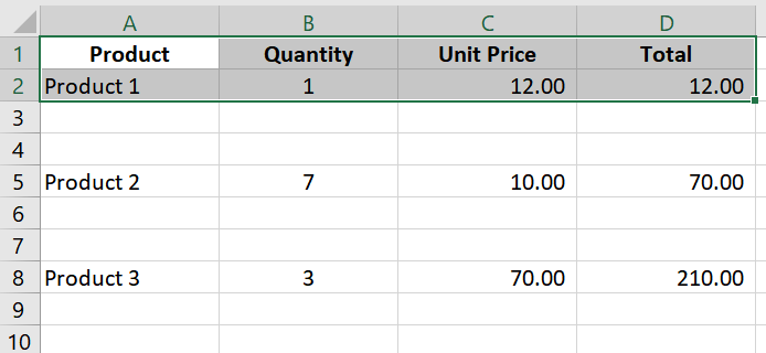
You can’t even select all the data by pressing CTRL + A. Notice that Excel doesn’t recognize the records after the blank rows as part of the data set.
With this data arrangement, you won’t be able to properly filter the records or even create charts.
In short, these blank rows are definitely making things difficult.
In this article, I’ll show you the quickest ways to solve this problem.
Method 1: “Go to Special” Option
To hide blank or null rows, the first step is to select the data set.
Since we can’t make use of CTRL + A to select it, we can do either of the following:
- Select the entire columns of the data set (as shown below).
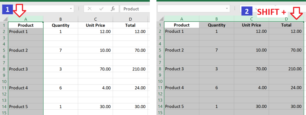
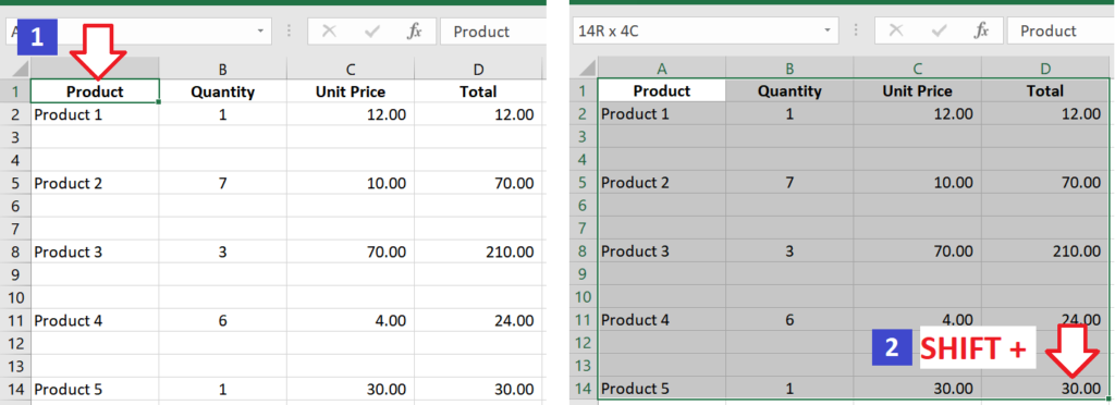
- Or, select the first cell and scroll down until you find the last cell of the data set.
Then, while pressing the SHIFT key, click on the last cell.
If you don’t have other data at the bottom of the data set, you may want to use the first option as that is the quickest way to select the cells.
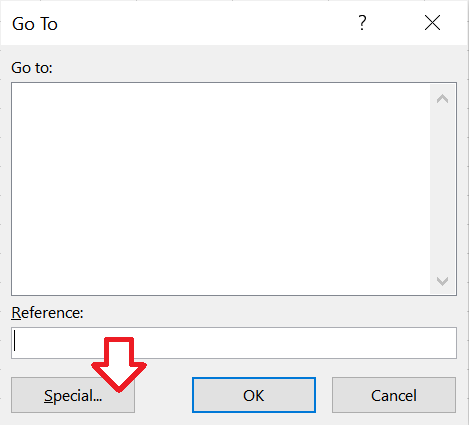
Once the cells are highlighted, press CTRL + G.
The Go To menu should appear. Once you see it, click on the Special… button.
You will then see the Go To Special menu. Select Blanks and click OK.
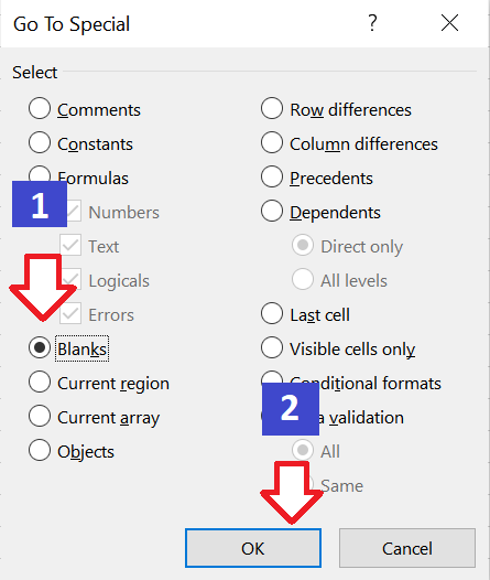
Note that the blank or null cells are highlighted.
Right click on one of these highlighted cells and select Delete…
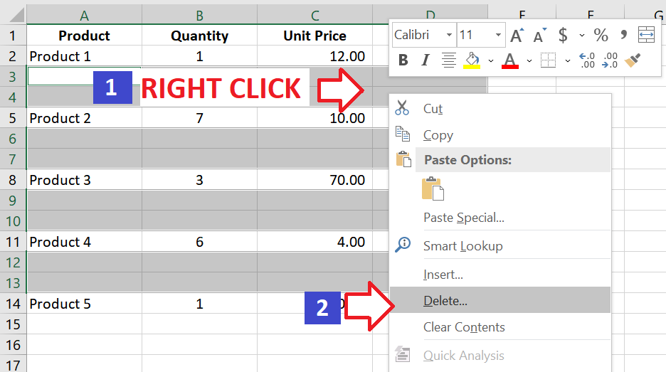
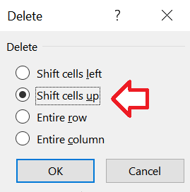
The Delete menu will appear. Select Shift cells up and press OK.
And voila! Blank rows are removed from your data set.
Method 2: “Auto Filter” Option
Another option to hide blank rows is to use the Auto Filter. Please know though that this option will require you to copy the data set to a different sheet or workbook. If this is ok with you, then this would be a good option for you too.
To use the Auto Filter, you must first select the cells within the data set.
Same as the steps specified above, you can either:
- Select the entire columns of the data set; or
- Select the first cell up to the last cell within the data set.
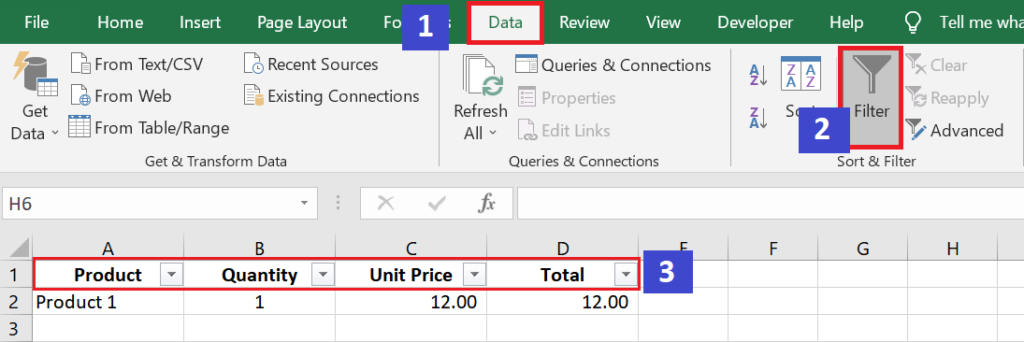
Once the cells are highlighted, apply the filters by going to the Data menu and selecting Filter.
You should then see the filters added to the header row.
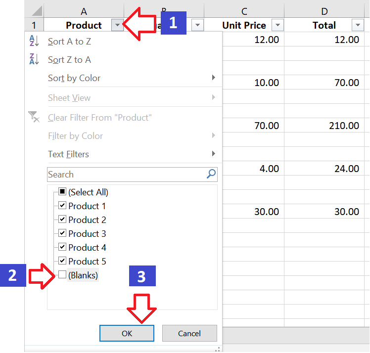
Once the filters are in place, add a filter so that the blank rows are excluded from the data set.
To do this:
- Select the filter in one of the fields.
- Uncheck (Blanks) – this will be the last item in the filters.
- Click OK.
You will now see the data set without the blank rows in between.
Once you see this, copy the filtered data (CTRL + C) set and paste (CTRL + V) it on a different sheet or workbook.
Conclusion
Blank rows within a data set are oftentimes inevitable especially when you’re dealing with exported data. But with just a few clicks, you can easily remove blank rows by either using the Go To Special or Auto Filter feature in Excel.