Excel is great at number operations and data analytics. However, when it comes to formatting of data, particularly text, you’d find Excel silent about quite a few things. For example, the strikethrough function.
Take a quick look around the Ribbon tab of your Excel workbook to see if something similar to a strikethrough button is visible? Don’t fret if you do not find it there. Unlike Microsoft Word, Excel doesn’t readily offer the strikethrough option through the Ribbon tab.
So what if you want some of your content in Excel to undergo the strikethrough formatting? You may want to do so to show revisions, finality, or cancellation of data etc.
Even though the strikethrough option is not visibly available in Excel, you can still use it in Excel. Also, you may add it to your Ribbon tab. Continue reading the article below to learn how.
Table of Contents
2 Ways to Strikethrough in Excel
You may add the strike-through formatting to your data in Excel through either of the following easy methods.
1. Shortcut Key (Ctrl + 5)
Let us begin with the easiest and the quickest way to get the strikethrough job done in Excel. Simple, use a hotkey.
Take a look here.
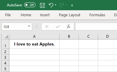
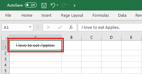
To strikethrough the sentence written in Cell A1, select it and press Ctrl+5. There it is, a line passes through the text in Cell A1 as shown below
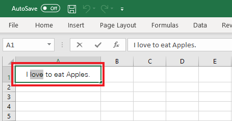
And what if you only want to strikethrough a certain word from the text in a cell and not the entire text?
Double-click the cell or press F2 to enter the Edit Mode, select the word to be strikethrough as shown below.
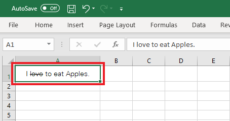
Once selected, press Ctrl + 5, and there you go.
2. Option to Format Cells
Select the cells where you want the strikethrough formatting added and right-click or use the shortcut key combination ‘Ctrl + 1’.
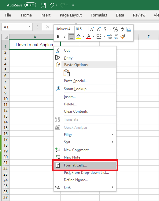
From the drop-down menu that opens up, select Format Cells as shown above.
This would take you to the ‘Format Cells’ dialogue box.
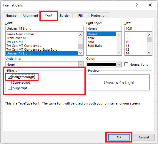
Under the tab Font > Effects > Check Strikethrough > Click ‘OK’
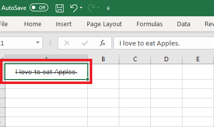
The results are as follows.
Adding the strikethrough button to your Ribbon Tab
Isn’t it a better option to ease the entire situation by adding a Go-to button to the Ribbon tab? Below are the steps that you need to follow to add a ‘Strike-through’ button to the Ribbon tab.
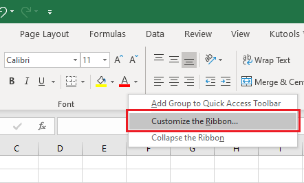
Step 1:
Click anywhere on the Ribbon tab to have the following dropdown menu opened and select ‘Customize the Ribbon’.
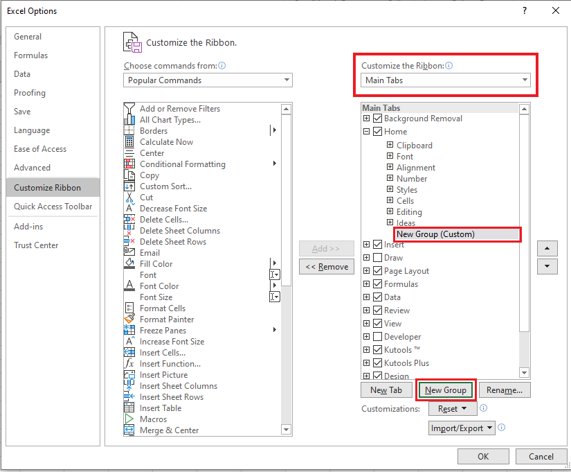
Under the head ‘Customize the Ribbon’ select ‘Main tabs’. Double click on Home to extend it down and click ‘New Group’ as highlighted below.
This would add a New Group to the Home Bar, where you can add custom buttons. Next, select ‘Commands not in the Ribbon’ from the ‘Choose Commands’ dropdown menu.
Under the Commands Box, select the Strikethrough function and click ‘Add’ to add it to the New Group.
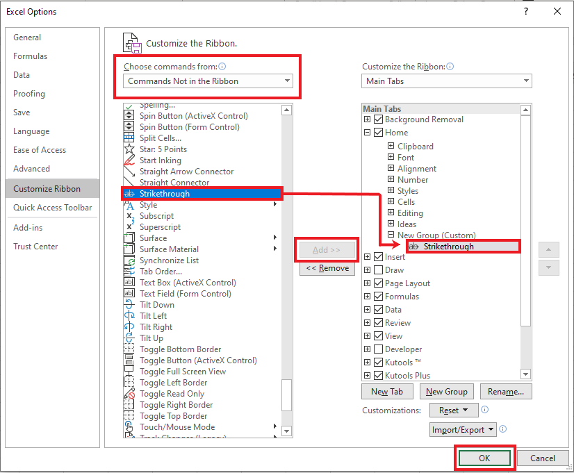
Click ‘Okay’ to see the button added to your Home Tab as follows.
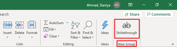
To strikethrough any data populated in a cell in Excel, simply select that cell and click the Strikethrough button as shown above.
If you use this function of Excel frequently, you may add the Strikethrough button to your Ribbon Bar. This not only saves time and effort but also rids you of the need to remember shortcuts and hotkeys.
Bottom Line
That is all about striking through data in your Excel sheet or adding a quickly accessible button to your Excel workbook. Keep coming back for more helpful articles.
Suggested Tutorial: How to Calculate Average in Excel?