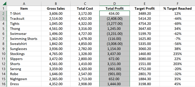
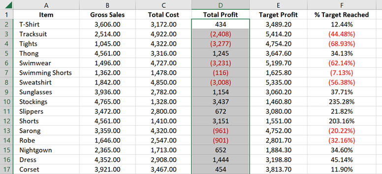
A negative percentage or a negative number is, by default, displayed in Excel with a dash or a negative sign in front of it. See the example below.
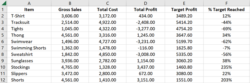
These dashes can go unnoticed when browsing a large dataset. That’s why some would prefer to have them enclosed in parentheses to let them immediately stand out.
This format makes it easier to distinguish the negative percentages or numbers from the positive ones.
In this article, I’ll show you how to change the cells’ format to display negative numbers and percentages inside parentheses.
How to Display Negative Numbers in Parentheses in Excel using the Number and Currency Format?
Note that his method only shows how to display negative numbers in parentheses. If you are looking for a way to surround the negative percentages in parentheses, please proceed to the next method.
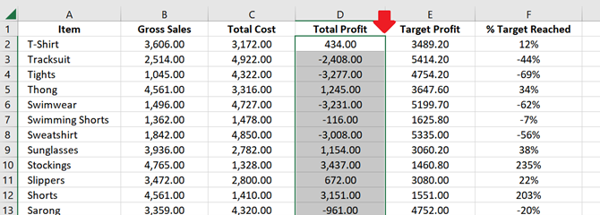
1. Select all the cells you want to format.
2. Go to the Home tab. Click the small arrow button next to the Number section (as shown below).
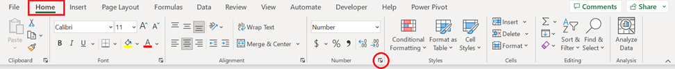
If you want the keyboard shortcut, simply press CTRL + 1.
3. The Format Cells menu will appear. Go to the Number tab.
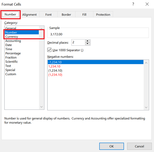
In the list of Categories, select either Number or Currency.
Select Currency if you want the currency symbol to appear in your cells. If not, choose Number.
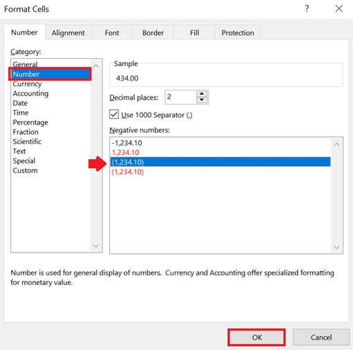
Once you have selected your desired category, you will see the Negative numbers section on the lower right of the menu.
This section allows you to select the format to apply to the negative numbers in the selected cells.
Select either the third or fourth option to enclose the negative numbers in parentheses.
If you want them in red font, select the fourth one. If not, choose the third one.
After selecting your desired format, click OK.
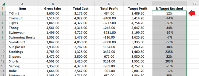
4. And that’s it! You should now have the negative numbers in your selected cells enclosed in parentheses.
How to Display Negative Percentages and Numbers in Parentheses in Excel by Creating a Custom Number Format?
This method works for both negative percentages and negative numbers.
1. Select all the cells you want to format.
2. From the Home tab, click the small arrow button next to the Number section (as shown below).
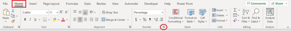
Or, if you like keyboard shortcuts, just press CTRL + 1.
3. The Format Cells menu will appear. Go to the Number tab.
From the list of categories, select Custom.
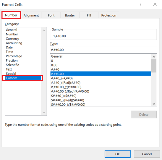
4. Next, we will write the custom number format.
But before we do that, I’ll walk you through the basics of writing one.
Excel accepts four parameters when writing a custom number format: [Positive Number]; [Negative Number]; [Zero]; [Text]
These four represent how you would like the cell to display a positive number, negative number, zero, and text respectively.
You don’t have to fill in all four. You only need to fill in whichever is necessary.
In our case, we only need to fill in the [Positive Number] and [Negative Number].
The next thing you need to know about custom number formats is the characters used to represent a number.
These are 0 and #. These two serve as the placeholder for a digit.
- 0 (zero) – use this to display 0 if its corresponding digit is blank or empty.
- # (hash, pound, or number sign) – use this to show a blank if its corresponding digit is blank or empty.
You can choose from the following formulas or use them as a guide in creating your own.
Negative Percentage enclosed in parentheses:
| Show only the whole number (no decimals) | 0%;(0%) |
| Always show two decimals | 0.00%;(0.00%) |
| Only show decimals if applicable | #.##%;(#.##%) |
Negative Percentage enclosed in parentheses in red font:
To highlight the negative percentages in red, you only need to add the word [Red] as a prefix for the [Negative Number].
| Show only the whole number (no decimals) | 0%;[Red](0%) |
| Always show two decimals | 0.00%;[Red](0.00%) |
| Only show decimals if applicable | #.##%;[Red](#.##%) |
Negative Numbers enclosed in parentheses:
| No decimals, with thousands separated by a comma | #,###;(#,###) |
| Always show two decimals, with thousands separated by a comma. | #,##0.00;(#,##0.00) |
Negative Numbers enclosed in parentheses in red font:
To highlight negative numbers in red, simply add the word [Red] as a prefix for the [Negative Number].
| No decimals, with thousands separated by a comma | #,###;[Red](#,###) |
| Always show two decimals, with thousands separated by a comma. | #,##0.00;[Red](#,##0.00) |
5. Enter your custom number format inside the Type textbox and click OK.

6. And that’s it! The negative numbers in your selected cells should now be inside parentheses.
What to do if the above solutions don’t work?
If the solutions above don’t work for you, it could be because of how your operating system (OS) is set up.
- If you’re using MAC, ensure that you have the latest version. Go to the App Store and click ‘Update’.
- If you’re using Windows, you will need to change the settings for the Negative Number Format and Negative Currency Format. You can try the following steps:
IMPORTANT: Before you start, please note that the following steps will affect all programs on your computer (not just Excel). Please remember the current settings applied so you can easily revert to them if needed.
The steps for changing these two settings slightly differ for each version of Windows (as shown in the following table).
| Windows 8 and Windows 10 | Windows 7 and Windows Vista | Windows XP |
| 1. Close the Excel file (and other Excel files that are open). | (same) | (same) |
| 2. Open the Control Panel. (You can search for it in the search bar next to the Start menu). | (same) | (same) |
| 3. Look for “Clock and Region”. | 3. Look for “Clock, Language, Region”. If you can’t find it in Windows 7, click Category in the View by menu at the top. | 3. Look for “Date, Time, Language, and Regional Options”. |
| 4. Click the link that says: “Change date, time, or number formats”. | 4. Click the link that says: “Change keyboards or other input methods”. If you’re in Classic view in Windows Vista, double-click “Regional and Language options”. | (same as Windows 7 and Vista) |
| 5. A menu will appear. From the Format tab, click the Additional Settings button at the bottom. | (same) | (same) |
| 6. Another menu will appear. From the Numberstab, find the Negative number format setting and change its value to (1.1). | (same) | (same) |
| 7. On the same menu, go to the Currency tab. Find the Negative currency format setting and change its value to ($1.1). | (same) | (same) |
| 8. Click OK on the two menus to apply the changes made. | (same) | (same) |
| 9. Open Excel and see if the settings were successfully applied. | (same) | (same) |
Conclusion
As you can see, enclosing negative percentages and numbers in Excel is a quick change in the cells’ number format. If, however, changing the number format doesn’t work, you may need to either update your OS (if you’re using MAC) or change the OS’ Regional Settings if you’re using Windows.