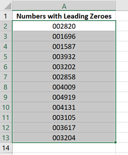
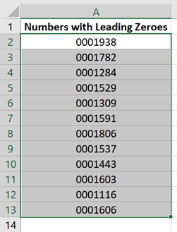
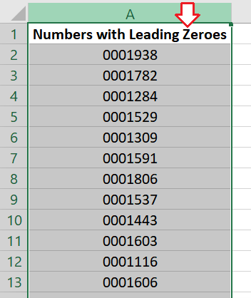
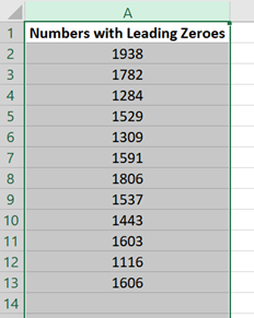
Excel, by default, automatically removes leading zeroes whenever you enter numbers. So, you might be wondering why there are leading zeroes in the Excel file you received.
Well, there are two possible reasons for that. It could be because:
- The cell is in text format.
This can happen if there’s an apostrophe at the start of the cell. Apostrophe (‘) is a special character that tells Excel to treat a cell as a text. If you are working on an Excel file exported from a system, there’s a great chance you’ll encounter this.
Remember that adding an apostrophe is just one way of converting a cell into a text. A cell can also be converted into text by simply changing its number format – so check on that too.
- The cell is formatted to have a fixed number of digits.
If you have a 3-digit number entered in a cell that was formatted to always have 5 digits, Excel will automatically fill in the missing 2 digits with leading zeroes.
There are plenty of ways to remove the leading zeroes in Excel. They vary depending on the reason for having them. I’ve arranged the methods below to tackle first the most common causes. I suggest you go through each of them and see what works on your data.
Error Check to Remove Leading Zeroes in Excel
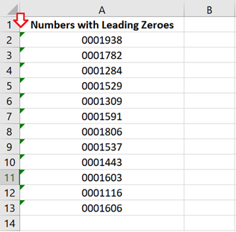
Excel will typically warn you if you have cells that contain numeric values but a formatted as text. You will notice this when you see small green triangles added on the left side of these cells (as shown below).
If you don’t see them, it’s most likely that Background Error Checking is disabled on your Excel.
To enable it, simply go to File >> More >> Options.

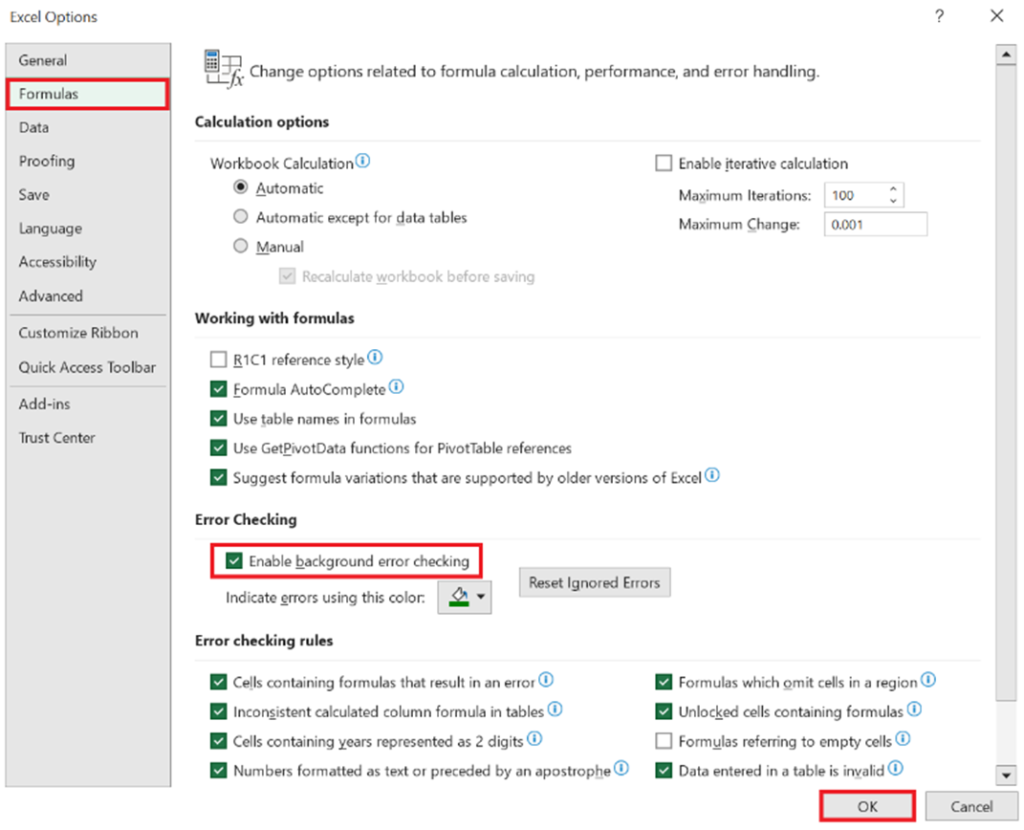
In the Excel Options menu, select Formulas.
Go to the Error Checking section, tick the “Enable background error checking” checkbox, and click OK.
You should now see the small green triangles on the left side of your cells.
(If you don’t see them still, please proceed to the method that follows after this).
Select all these cells, and a yellow warning icon will crop up on the first cell selected.
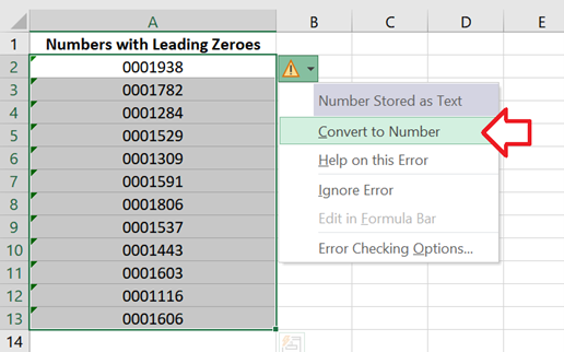
Click on that icon and select Convert to Number.
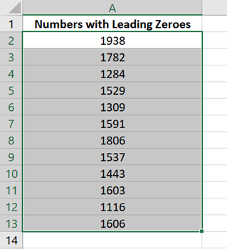
And that’s it! All leading zeroes should now disappear.
With this approach, we have taken advantage of Excel’s default setting of removing leading zeroes from numbers.
Changing the Number Format to Remove Leading Zeroes in Excel
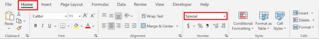
If the previous method didn’t work for you, it might be because your cells are in a “Special” format where leading zeroes are automatically added so that it reaches a particular number of digits.
To change this:
1. Select all the cells with leading zeroes.
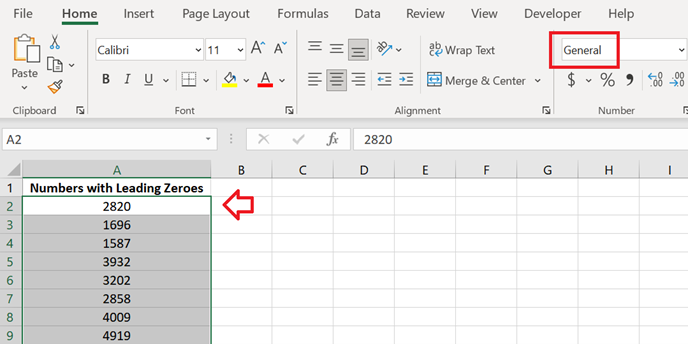
2. Go to the Home tab. Look at the current number formatting of these cells from the Number Section. If it is “Special”, change the number formatting to General (or any other number formatting appropriate for your data).
And that’s it! You should no longer see any leading zeroes in your selected cells.
Using “Paste Special” to Remove Leading Zeroes in Excel
If you don’t want to alter the cells containing leading zeroes and would only want the numbers on a different column, then you can do the following:
1. Select a blank cell on the worksheet and press CTRL + C to copy it.
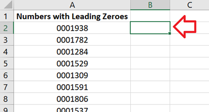
2. Next, select all the cells with leading zeroes.
3. Then, press CTRL + ALT + V to open the Paste Special menu.
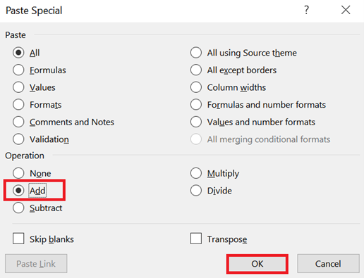
Select Add under the Operation section and click OK.
And that’s it! You should now have removed all the leading zeroes from your cells.
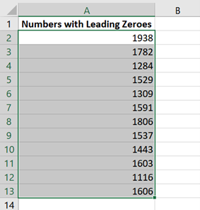
This method worked because it added a zero (or a blank cell) to all the cells with leading zeroes, which in the process, converted the cells into numbers.
Using the VALUE Function to Remove Leading Zeroes in Excel
Another way to remove leading zeroes without altering the original column is to use the VALUE() function.
VALUE() is a text function in Excel that converts a text string that looks like a number into an actual number.
On a new column, type the following formula: =VALUE([range])
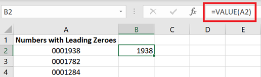
As you press enter, the leading zeroes will disappear.
Copy this formula to the remaining rows, and voila! No more leading zeroes for the entire column.
Using Text to Columns to Remove Leading Zeroes in Excel
If you have a lot of rows to remove the leading zeroes from, this may be the best option for you.
1. Highlight the entire column that contains leading zeroes.
2. Go to the Data tab. From the Data Tools section, click Text to Columns.

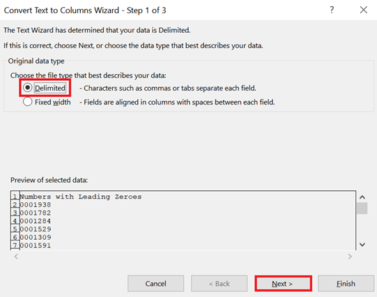
3. The Convert Text to Columns Wizard will appear.
Select Delimited and click Next.
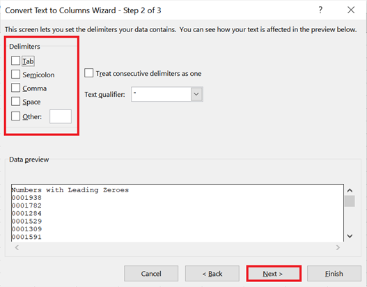
4. Uncheck all the Delimiters checkboxes and click Next.
5. In the Column Data Format, select General.
Notice there’s a note in the Wizard that says:
'General' converts numeric values to numbers, date values to dates, and all remaining values to text.
This is the Text to Column feature that we are making use of.
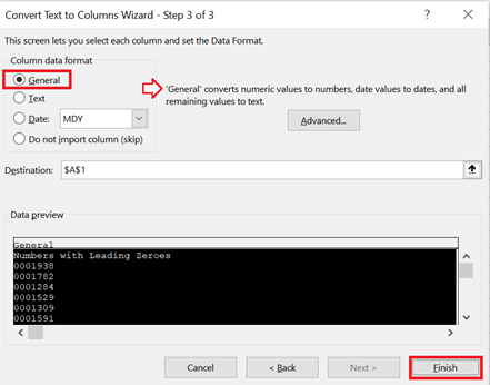
Click Finish to close the Wizard.
You should now see all the leading zeroes removed from your selected column.
If you have used Text to Columns before and worry that this may affect other columns alongside the current field, don’t worry. Only the selected column gets updated with the settings we selected in the Wizard.
Remove Leading Zeroes from an Alphanumeric Data
The methods described above involved the conversion of the cell into a number format.
If you are working on data with alphanumeric characters (a combination of both letters and numbers) and you only want to remove the leading zeroes, then this next method is for you.
1. On a blank column, type this formula:
=RIGHT(A2,LEN(A2)-FIND(LEFT(SUBSTITUTE(A2,"0",""),1),A2)+1)Change all instances of “A2” with the range where your alphanumeric data is.
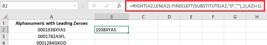
2. Once you click enter, the cell should result in an alphanumeric character with no leading zeroes.
3. Copy this formula to the remaining rows in your cells, and you’re all set up.
Conclusion
Leading zeroes are often intentionally added for a particular purpose. However, there are instances when we need to remove them. I hope the methods provided above have helped you do so with ease.