How to Swap Columns in Excel?

When working with a data set, there will be times when you need to rearrange the columns. These can occur whenever you need to compare similar fields side by side.

In this article, I’ll show you 4 different ways that you could do to move or swap columns while keeping your data intact.

Method 1. Drag and Drop

If you are looking for the quickest way to move columns, the drag-and-drop option is definitely on top of the list.

Note, however, that this will only work if you have only one set of data in the worksheet.

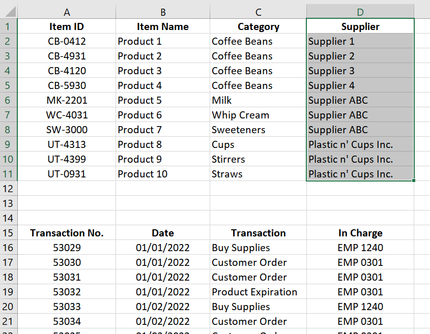
If you have more than one group of data in your worksheet, say you have a product list on top and a transaction list at the bottom, use the Cut and Paste method outlined below.

Here are the steps to do a column drag and drop:

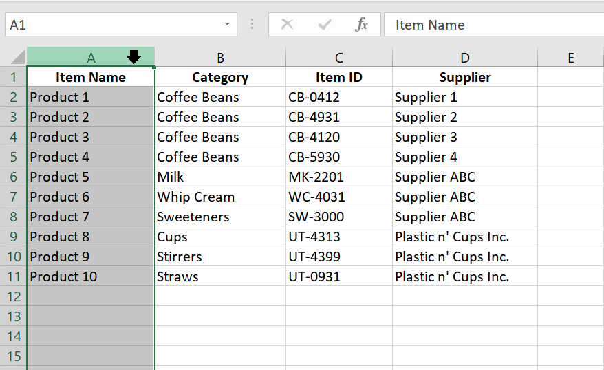
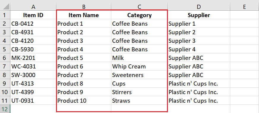
1. Select the entire column that you’d like to move.

You can do this by hovering your mouse on the column letter on top of the column. Wait until the mouse cursor changes into a black arrow. Once you see that, left-click on your mouse.

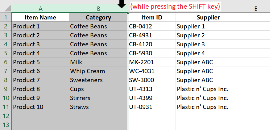
If you want to also move the columns next to it, while pressing on the SHIFT KEY, click on the column letter of the last column that you’d like to include.

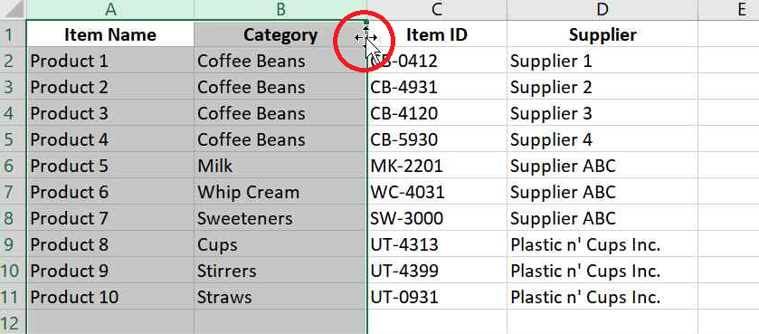
2. Once you have selected the column(s) that you would like to move, hover your mouse to the right side of the selection. Wait until you see your cursor change into an arrow cross.

3. While pressing on the SHIFT KEY, drag the arrow cross to the area where you would like to place the selected column(s). As you move your cursor over the columns, notice that a green bar (|) will appear. This bar will tell you where your columns will go.

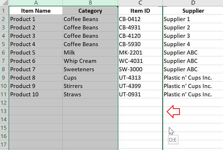
Once you arrive at your desired spot, release your mouse. You should now see your column(s) moved.

Important:

Before dragging the selected column(s), ensure that you are pressing on the SHIFT KEY the whole time. Pressing on this key signals Excel to move the columns.

Otherwise, Excel will overwrite the contents of the cells on the selected spot.

If the spot (or column destination) that you have selected has existing data in it, you will see this warning:

Select Cancel to redo the process.

Method 2. Cut and Paste

This method allows you to select the cells you would like to move.

You could either:

• move the entire column; or
• only move a selected group of cells

Use this if you are working on a worksheet with multiple datasets. This approach ensures that the other datasets are not affected by your changes in one.

To do this:

1. Select the entire column or group of cells that you want to move.

2. Right-click on the selected cells and select Cut.

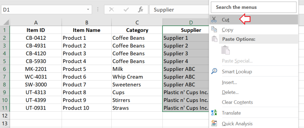
Or, you could use the keyboard shortcut by pressing CTRL + X.

3. Once you see the broken lines surrounding the selected cells, click on the topmost cell where you would like to move the selected cells to. Right-click on it and select Insert Cut Cells from the menu that appears.

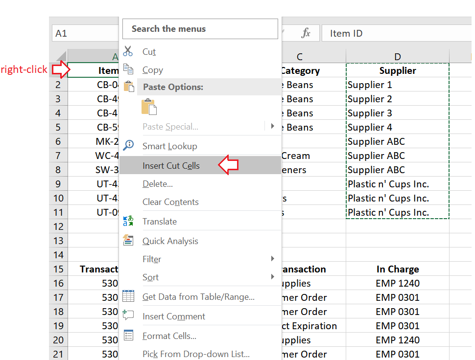
And that’s it! Your chosen columns or cells should now move.

Method 3. Sorting

This method is your best option if you have to reorder ALL the columns in your data set.

To swap the columns using the Sort method:

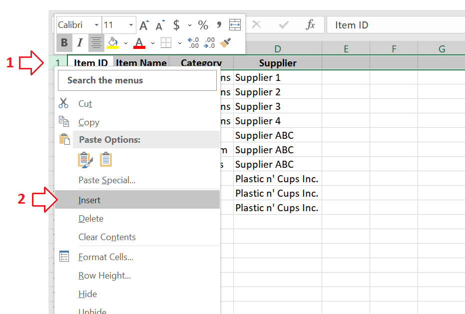
1. Insert a new row above your data set – right above your headers.

If you have a blank row already, you can skip this step.

Right-click on the entire header row and select Insert from the menu.

2. Enter a number above each header – this will serve as the basis for the order of the fields.

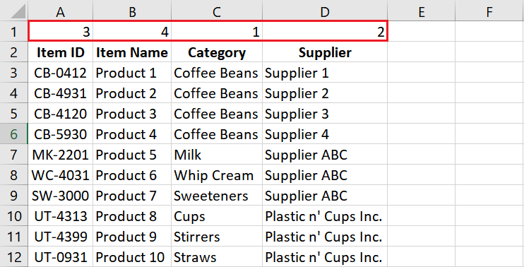
Once you’re all set with the order of the fields, the next step is to apply the sorting.

3. Highlight your entire data set by selecting just one cell from the data set and pressing CTRL + A.

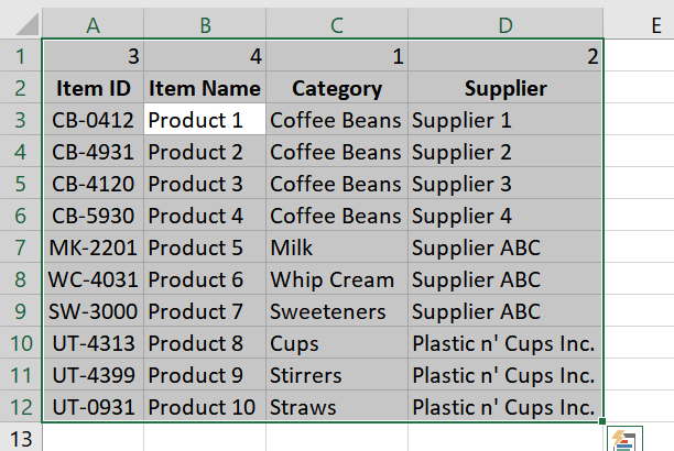
Remember to include the numbers that appear above the headers.

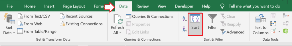
4. Go to Data >> Sort & Filter section >> Sort

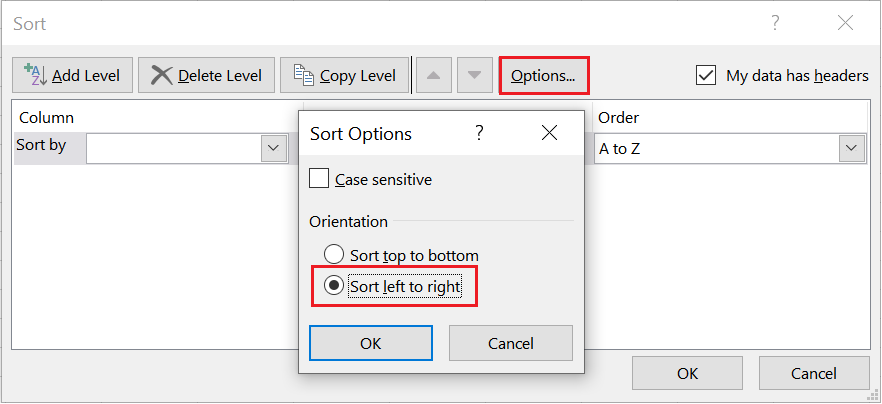
5. In the Sort menu, click on the ‘Options…’ button.

From the Sort Options, select ‘Sort left to right’ and click OK.

6. For the Sort By option, select the row where you’ve placed the sort numbers.

In my example, it’s in Row 1.

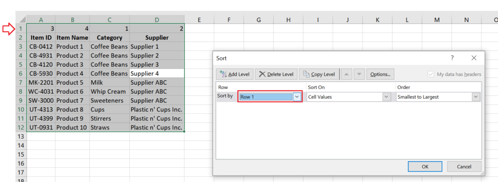
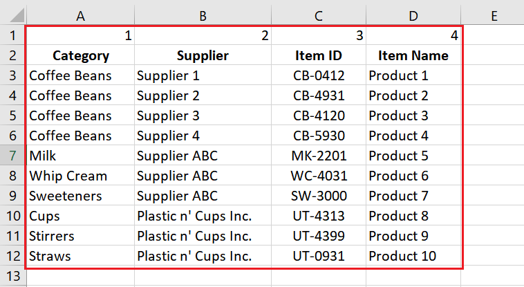
7. Click OK. You should now see your data set rearranged based on your sort numbers.

Method 4. Using VBA

If you frequently change the arrangement of the columns in your data, you might want to use a macro to automate this time-consuming task.

Note that this strategy only works when the fields in your data are in a fixed sequence.

ThisWorkbook.Activesheet.Columns("A:A").Cut
ThisWorkbook.Activesheet.Columns("C:C").Insert Shift:=xlToRight

The code above moves the entire column A to column C in the active worksheet.

Copy these two lines of code in your module.

Remember to update the column range specified within the double quotes (“).

If you want to move multiple adjacent columns at one time, you could configure your code to look something like this:

ThisWorkbook.Activesheet.Columns("A:C").Cut
ThisWorkbook.Activesheet.Columns("D:D").Insert Shift:=xlToRight

The code above moves columns A and B to column C.

If you need to move another set of columns, copy the two lines of code as many as necessary, and make the appropriate edits.

Conclusion

Knowing how to switch columns is crucial when working on a dataset. Choose from the four strategies mentioned and see what best suits your needs.

Also Read: Remove Duplicates Based on One Column in Excel