Have you ever tried writing a formula that worked well on one cell, but when you copied and pasted it to other cells, it no longer worked as expected? That could be a sign that you need to anchor at least one of the cells referenced in your formula.
In this tutorial, I will show you how to anchor cells and explain the significance of the dollar sign ($) that you see in formulas. If you are new to Excel, please know that the dollar sign does not mean money or the dollar currency in an Excel formula. It’s what we use to anchor the cell.
Table of Contents
What is a Cell Anchor?
To “anchor a cell” essentially means to convert a relative cell reference to an absolute cell reference. In other words, it locks or anchors the reference to a specific cell (or group of cells).
When we create formulas, Excel, by default, sets a relative reference to the cells.
A formula has a relative cell reference when it does NOT contain any dollar sign ($) (as shown in the example below).
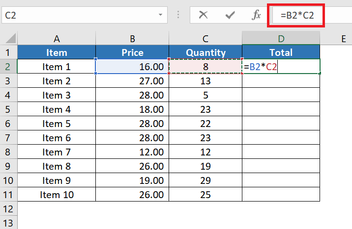
When we copy this kind of formula to other cells, the cells referred to change based on the relative position of rows and columns.
In the example above, cell D2 has this formula: =B2*C2.
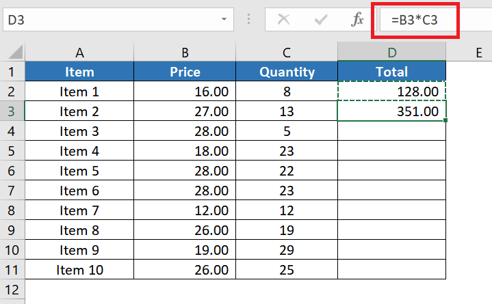
If I copy the cell and paste it on cell D3, the formula becomes =B3*C3.
(Notice that the row number has changed).
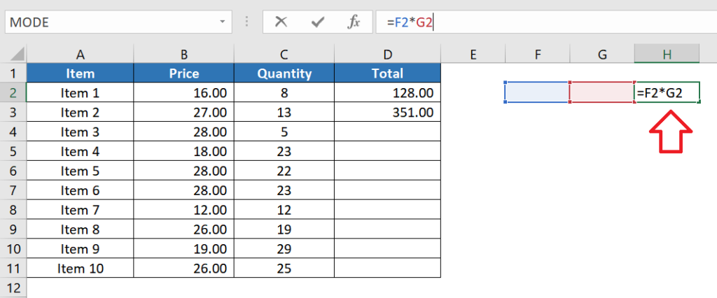
If I copy it on a different column, for example, cell F2, the formula becomes =F2*G2.
(Notice now that the column has changed).
Use formulas with relative cell references if your goal is to apply the same formula pattern in other cells.
On the other hand, if your goal is to have a fixed reference to a particular cell, add an absolute cell reference. This is when you will need to anchor the cell.
Anchor a Cell in Excel
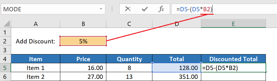
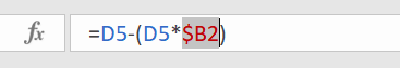
1. The first step is to write your formula in one cell.
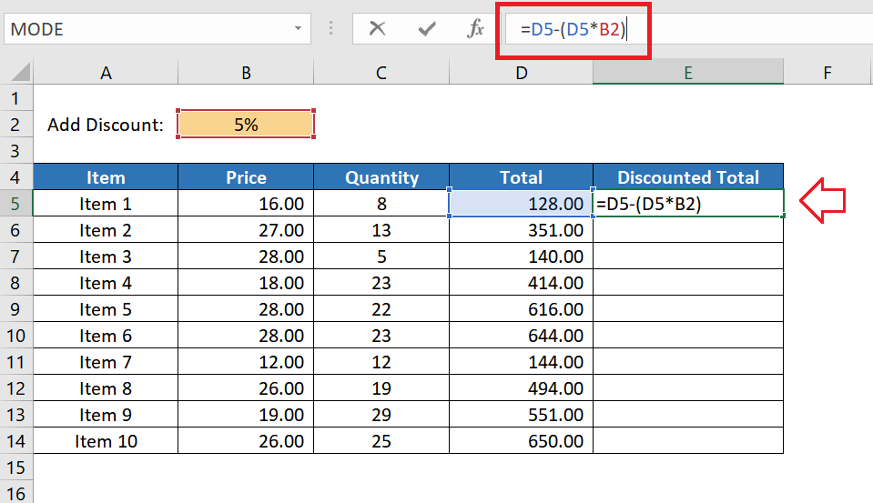
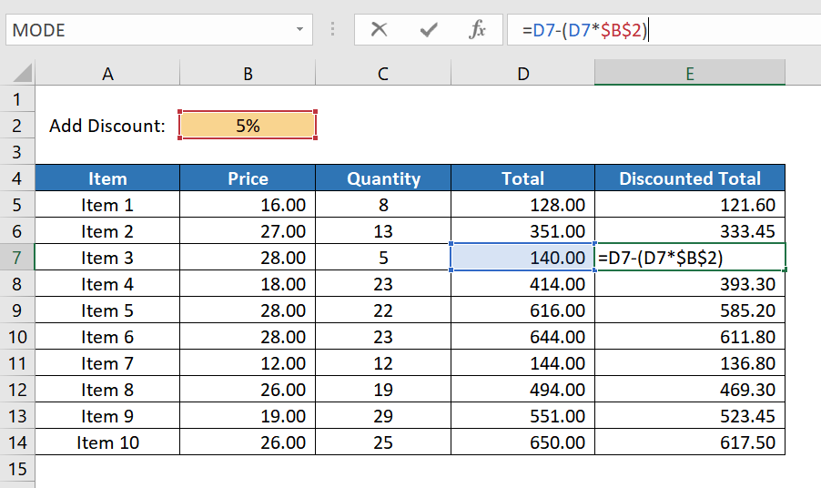
In the example above, I created a formula that gets the discounted total.
Notice that the formula doesn’t have any dollar sign ($) yet.
2. Once you get your formula working, the next step is to identify which cells in your Excel formula require an absolute reference.
In my example, there should be a fixed reference to cell B2 — where the discount percentage is stored.
3. Once you have identified the cells that require fixed references, it’s time to add the dollar sign ($).
Note that there are three types of absolute cell references.
| Type of Absolute Reference | Example |
| Fixed row and column | =$A$1 |
| Fixed row only | =A$1 |
| Fixed column only | =$A1 |
If you add a dollar sign before the column, it means the column will not change.
If you add a dollar sign before the row number, it means the row number will remain the same.
In my example, I need to add the dollar sign to both the row and column because the value I intend to use in the formula should always come from the same cell.
You could type the dollar sign ($) within the cell address(es) in your formula, but that could be too burdensome if you have a lot of cells that require an absolute cell reference.
The quickest way to do it is by pressing the F4 key.
From the formula bar, click on the cell that requires an absolute reference. You can also move the cursor to anywhere near that cell.
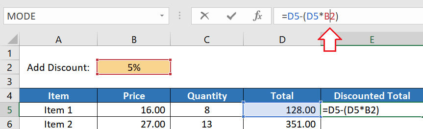
After that, press F4.
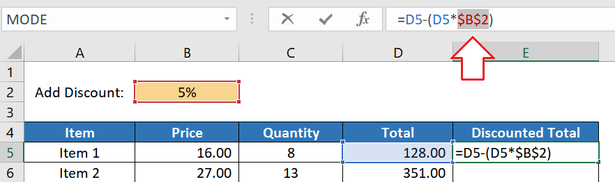
Notice that Excel automatically adds the dollar sign on both the column and row.
Press F4 again and notice that the dollar sign only appears on the row.
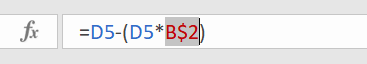
Press it again and notice that the dollar sign is only on the column.
Press F4 again and notice that the dollar signs ($) are removed from the cell – making it a relative cell reference.
Keep on pressing F4 until you see your desired cell reference. If you’re happy with the result, press ENTER to keep your changes.
Repeat the same steps for other cells in your formula that needs an absolute reference.
4. Once you have added all the necessary absolute references, try copying the cell with the formula to other cells. If correctly set up, the calculations should now work even on other cells.
Anchor Multiple Cells at One Time
If you have multiple cells in your formula that you want to anchor in one go, you can do the following:

In my example above, I highlighted all the cells inside the formula.
2. Once highlighted, press F4. Press on it again until you see your desired type of anchor.

In my example, I wanted to have two types of anchors in my formula:
- Anchor in the column only for cell D5
- Anchor in both the row and column for cell B2
It would be easier if I only highlighted cells D5 and pressed F4 to add an anchor. Excel, however, does not allow you to change the anchors of cells that are not in the same parentheses.
Since this is the case, I opted to highlight all of the cells in the formula and pressed F4 until I added an anchor to cell D5. After that, I highlighted cell B2 and pressed F4 until the appropriate anchor for it appears

Conclusion
When writing formulas in Excel, it’s crucial to know when to use a relative cell reference and when to use an absolute cell reference. Shifting from a relative to an absolute cell reference (or vice versa) is as easy as adding and removing the dollar sign ($) in the formula. I hope the tips provided above will help you do this with ease.