Decimals, fractions, and percentages are all ways to describe parts of a whole.
Percentages, however, are preferred by many over other formats. I guess it’s because whole numbers (with a percent sign at the end) are easier to interpret over decimals and fractions.
In this article, I’ll show you ways to convert decimals to percentage format in Excel.
Even though the steps are pretty straightforward, there’s one crucial thing we must first understand. We must know how Excel converts decimals to percentages. Skipping this step may result in us not getting the result we want.
By default, Excel converts a decimal by multiplying it by 100 and adding the percent sign at the end of it. If you are only looking for a way to add the percent sign at the end of your pre-calculated decimals (and not multiply them by 100), don’t worry. There’s a method for that too.
I have split this article into two methods:
- The first one converts the decimals to percent by multiplying them by 100 before adding the percent sign.
- The second one only adds the percent sign at the end of the decimals.
How to Convert a Decimal to Percentage in Excel?
Note that this method will multiply the decimals in your cells by 100. Let’s say you have 0.53 as your decimal. With this method, the resulting percentage will be 53%.
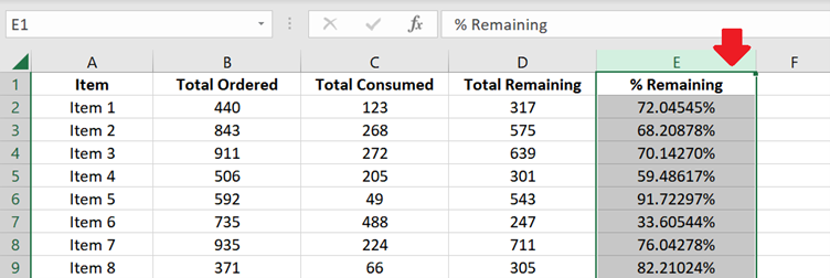
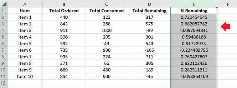
1. Select the cells containing the decimals you want to convert into percentage format.
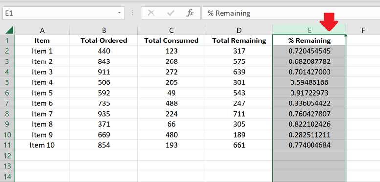
If you like, you can also select the entire column where these decimals reside by selecting the appropriate column letter on top (see the example above).
This way, the numbers you will enter later will be automatically converted into percentage format.
2. Next, proceed with one of the methods described below. Each of them has its advantage over the others. So, I suggest you read them all to find the most appropriate method for your situation.
Convert Decimal to Percentage in Excel Using the Percent (%) button from the Home tab
The quickest way to convert decimals to percentages is to go to the Home tab and click on the % (percent) button in the Number section.
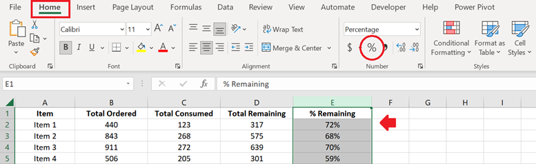
If you want the keyboard shortcut, you can press CTRL + SHIFT + %.
That’s it! Your numbers are now converted into percentages.
By default, the percentages will not show any of the decimals.
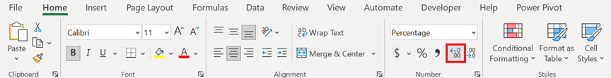
If you want to have some of the decimals visible, simply click on the “Increase Decimal” button (the second rightmost button in the Number section). Click on it as many times as you want. A single click corresponds to one decimal added.
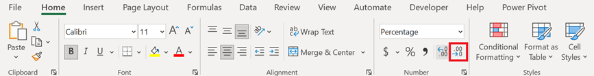
On the other hand, if you want to decrease the number of decimals shown, click on the “Decrease Decimal” button. Like the “Increase Decimal” button, a single click corresponds to one decimal removed.
Convert Decimal to Percentage in Excel using the Format Cells menu
This method is the “traditional way” of converting a cell’s format to a percentage.
From the Home tab, click on the small arrow button on the right side of the Number section.
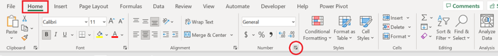
If you want the keyboard shortcut, simply press CTRL + 1.
The Format Cells menu will appear.
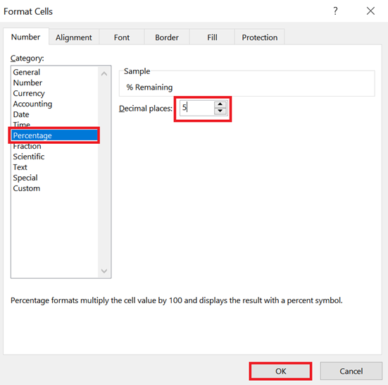
From the list of Categories, select “Percentage”. Type the number of decimal places you want to appear and click OK. That’s it!
What’s great about this method is that it allows you to enter the number of decimals you intend to include. There’s no need to click the “Increase/Decrease Decimal” buttons multiple times to adjust them.
Convert Decimal to Percentage in Excel using a Custom Number Formatting
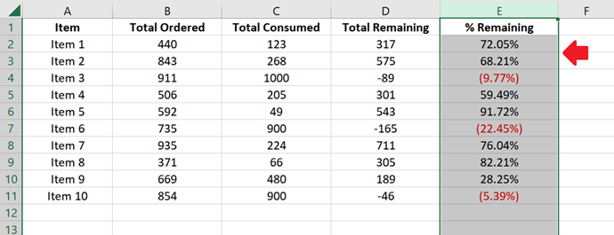
This method is perfect if you want the negative percentages to stand out from your dataset. Here, you get to decide how to format them. You could enclose them in parentheses and have them in red font.
1. Open the Format Cells menu by pressing CTRL + 1.
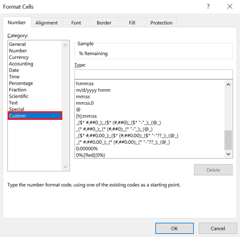
2. From the list of Categories, select “Custom”.
3. In the Type textbox, we are going to enter the Custom Number Formatting.
You can choose from the following custom number formats or use them to create your own.
| 0%;(0%) | No decimals are displayed; Negative percentages are enclosed in parentheses. |
| 0.00%;(0.00%) | Two decimals are displayed; Negative percentages are enclosed in parentheses. |
| 0%;[Red](0%) | No decimals are displayed; Negative percentages are enclosed in parentheses and are in red font. |
| 0.00%;[Red](0.00%) | Two decimals are displayed; Negative percentages are enclosed in parentheses and are in red font. |
The first two parameters in a custom number format are: [Positive Number]; [Negative Number].
Zero (0) serves as the placeholder for a digit. So, if you want to add more decimal places, simply add more zeroes after the decimal point.
[Red] represents the red font color applied.
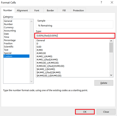
4. Once you’ve entered your custom number format in the Type textbox, click OK.
That’s it! The cells that you have selected should now be formatted as percentages, with the negative percentages enclosed in parentheses and/or highlighted in red font.
How to Add the Percent Sign (%) at the End of a Decimal?
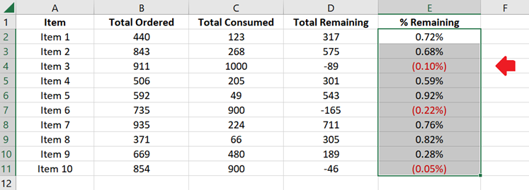
Note that this method will retain whatever number is in the cells and will only add the percent sign at the end of each. So, if you have 0.53 as the decimal, the resulting percentage will be 0.53%.
1. Select the cells where you would like to add the percent sign.
2. From the Home tab, click the down arrow of the dropdown list under the Number section and select More Number Formats.
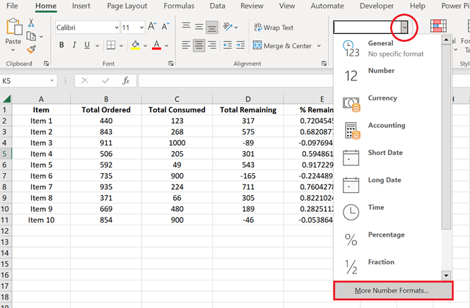
(If you like, you can also just press CTRL + 1 for the keyboard shortcut.)
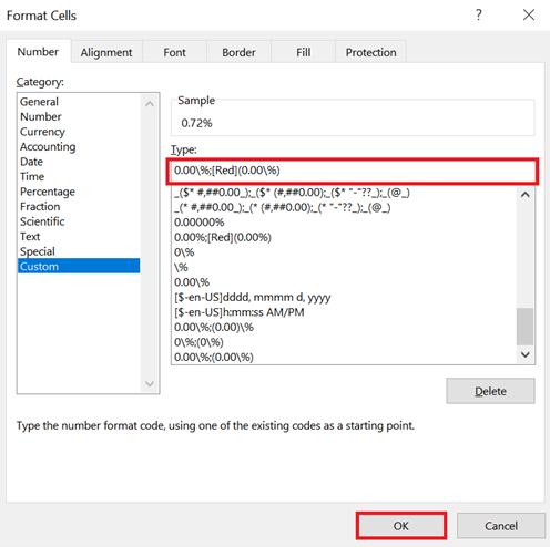
3. The Format Cells menu will appear. From the list of Categories, select “Custom”.

4. In the Type textbox, enter either of the following custom number formats.
| 0.00\%;(0.00\%) | Two decimals are displayed; Negative percentages are enclosed in parentheses. |
| 0.00\%;[Red](0.00\%) | Two decimals are displayed; Negative percentages are enclosed in parentheses and are in red font. |
In case you’re not yet familiar with custom number formats (or if you haven’t read the other methods described above):
- The first two parameters in a custom number format are: [Positive Number]; [Negative Number].
- Zero (0) serves as the placeholder for a digit. So, if you want to add more decimal places, simply add more zeroes after the decimal point.
- [Red] represents the red font color applied.
The backslash (\) in the custom number formats is a special character that tells Excel to simply add the percent sign and not convert the numbers by multiplying them by 100.
After entering your custom number format in the Type textbox, click OK.
5. And that’s it! The percent sign should now be added at the end of your decimals.
Conclusion
As you can see, there are plenty of ways to convert your decimals into percentage format. But you must first identify whether you only need to add the percent sign (%) at the end of your decimals or you need to have them multiplied by 100 to properly convert them.
You can go to the next tutorial: Round up Decimals to Nearest Whole Number