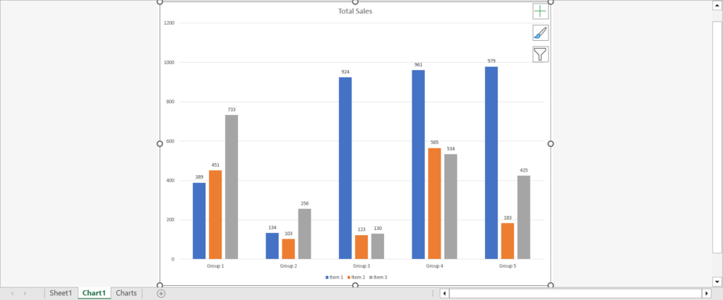
Charts are a great way to visualize data. Since we’re dealing with visualizations, the placement of these charts also matters. Oftentimes, it’s better to separate the raw data from the charts to make our dashboards clean and more appealing. In this article, I’ll show you ways to do just that.
Move the Chart to a New Sheet as a Chart Object
To move the chart to a new sheet as a chart object:
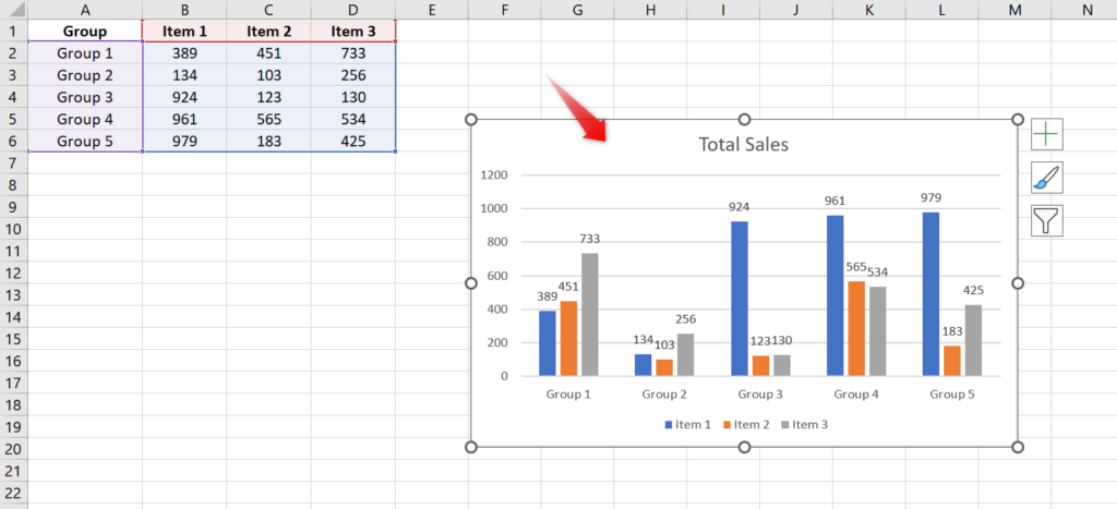
1. Click on a blank space on your chart to select it.
2. Once the entire chart is selected, click Chart Design from the Excel ribbon.
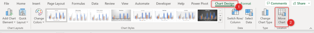
Go to the Location section and click Move Chart.
3. The Move Chart menu will appear.
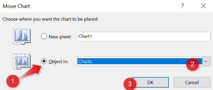
Tick the Object in option.
From the dropdown menu, select the sheet where you want to move the chart and click OK.
NOTE: If you haven’t yet added that sheet, close the menu first, insert a new sheet, and redo the steps.
4. Once you click OK, you will be redirected to the specified sheet.
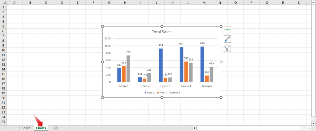
You’ll then see the chart that you have previously selected.
Drag the chart to wherever you like to position it inside that sheet. And that’s it! You’re all set.
Move the Chart to a Chart Sheet
If you prefer a designated sheet for your chart, then it would be best to move the chart to a Chart Sheet.
A chart sheet is like a regular worksheet, except that a chart sheet has no gridlines, making it easy to read through the chart.
The chart inside it is also magnified and centered. Anyone can easily go over it.
The chart cannot be resized by the users. It cannot even be deleted. If you want to delete the chart, you must delete the sheet itself because it is directly linked to it.
Setting up a chart sheet is perfect if you want your target audience to be able to focus on the chart and examine it without any distractions.
To move your chart to a chart sheet:
1. Right-click on the chart. When the pop-up menu appears, select Move Chart.
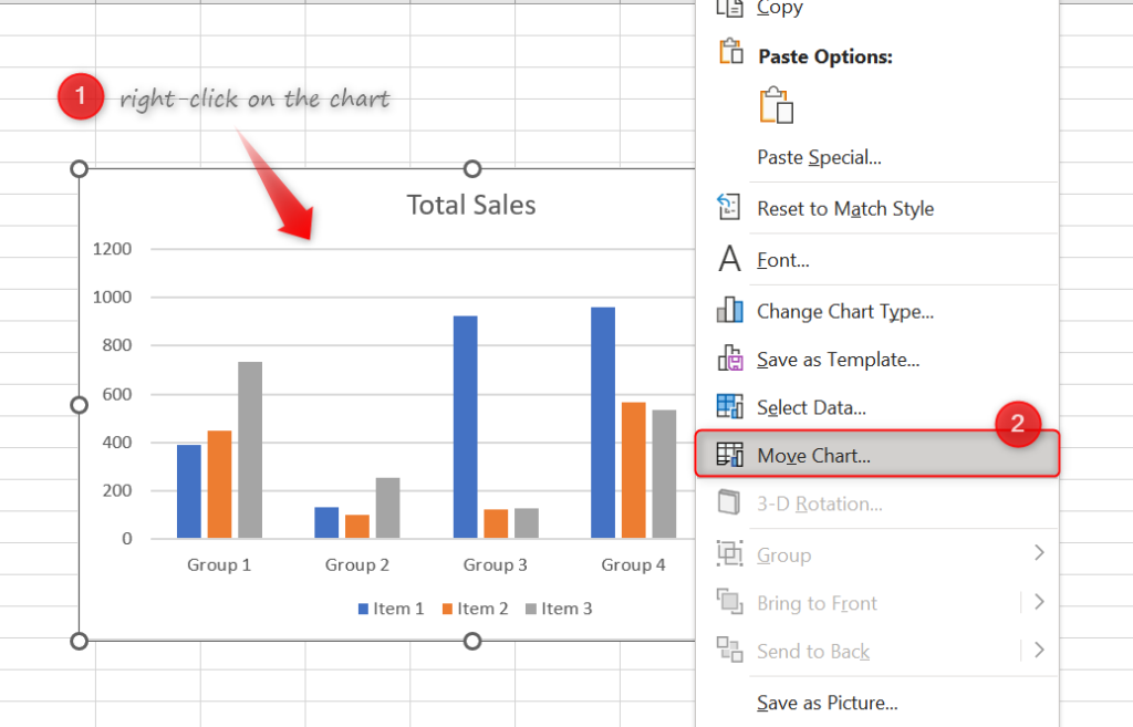
2. The Move Chart menu will appear.
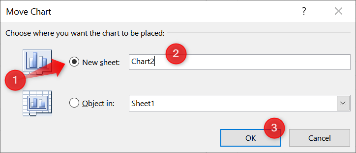
From the list of options, select New Sheet.
Enter the name you want for this chart sheet and click OK.
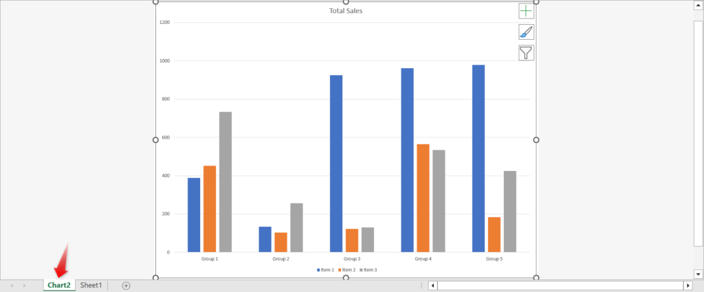
3. And that’s it! You now have your chart added to a chart sheet.
Move the Chart to a New Sheet Using the Cut and Paste Method
If you prefer doing things with keyboard shortcuts, then you will like this method.
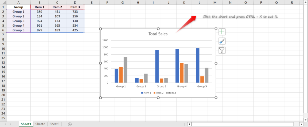
To transfer a chart from one sheet to another, simply select the chart and press CTRL + X to cut it.
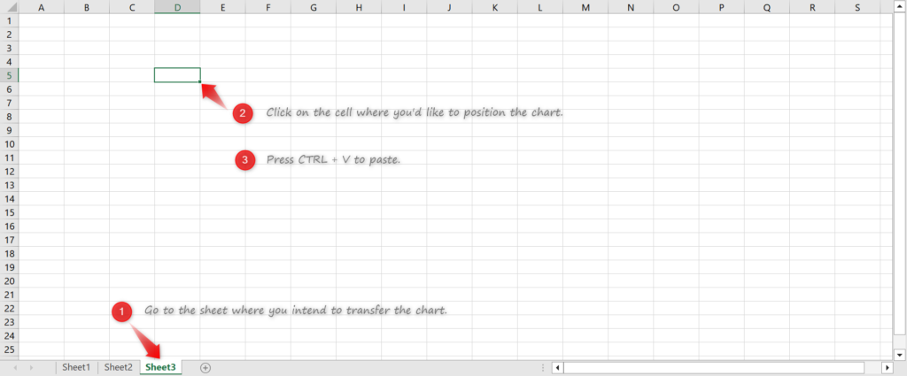
Once it’s cut, go to the sheet where you’d like to transfer it.
Click on the cell where you’d like to position your chart. Once selected, press CTRL + V to paste.
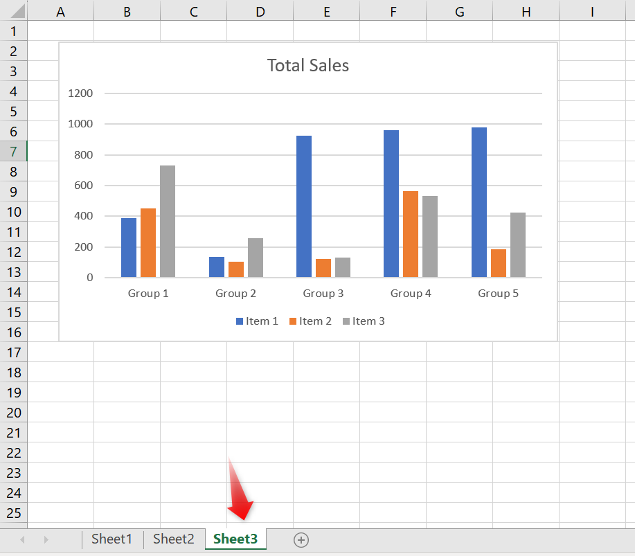
And that’s it! You have successfully transferred the chart onto the new sheet.
Move Multiple Charts to a New Sheet in One Go Using VBA
If you have multiple charts spread throughout different sheets in your workbook and you want to place them all in just one sheet, then this method is perfect for you.
This approach is great for creating a dashboard because you can transfer all sheets in one go. No need to go through each sheet to transfer each of them.
To do this:
1. While your workbook is open, press ALT + F11 to open the VBA Editor.
2. Then, from the Insert menu, select Module.
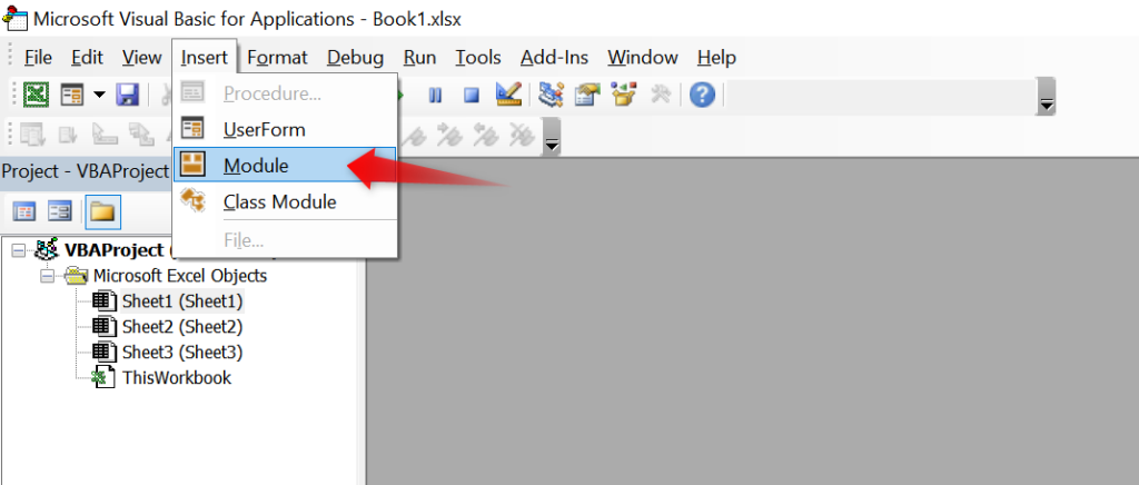
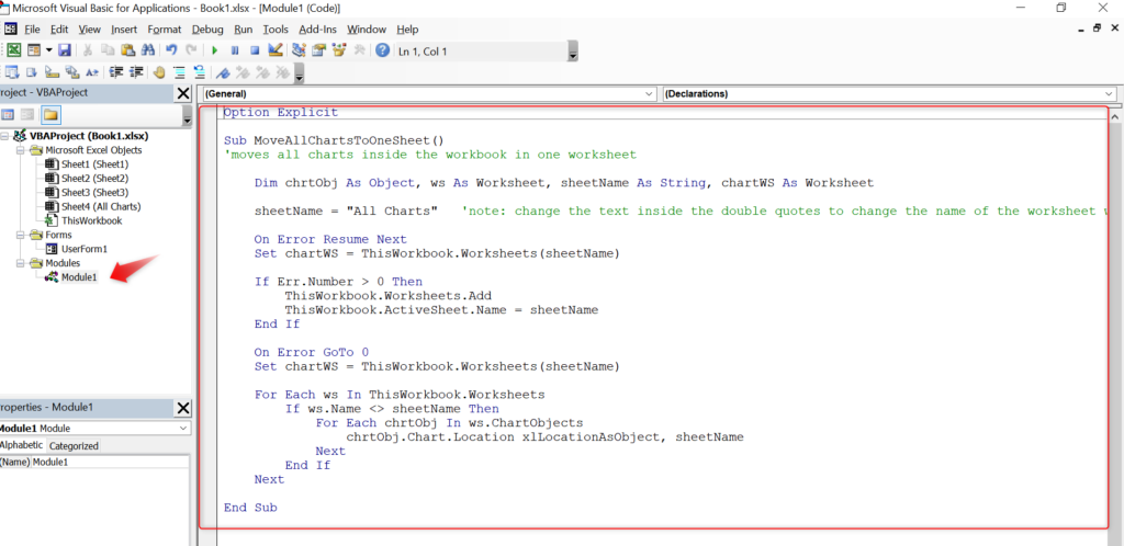
3. Copy the following code and paste it onto the new module added.
Option Explicit
Sub MoveAllChartsToOneSheet()
'moves all charts inside the workbook in one worksheet
Dim chrtObj As Object, ws As Worksheet, sheetName As String, chartWS As Worksheet
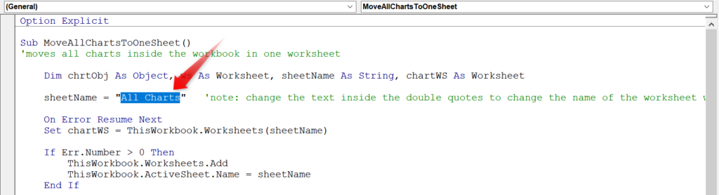
sheetName = "All Charts" 'note: change the text inside the double quotes to change the name of the worksheet where all charts will be moved to.
On Error Resume Next
Set chartWS = ThisWorkbook.Worksheets(sheetName)
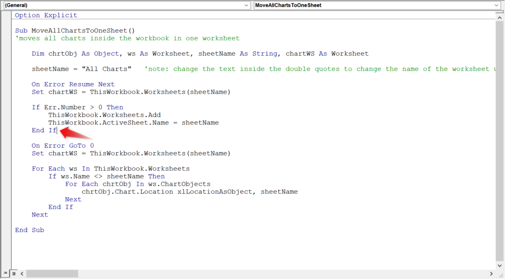
If Err.Number > 0 Then
ThisWorkbook.Worksheets.Add
ThisWorkbook.ActiveSheet.Name = sheetName
End If
On Error GoTo 0
Set chartWS = ThisWorkbook.Worksheets(sheetName)
For Each ws In ThisWorkbook.Worksheets
If ws.Name <> sheetName Then
For Each chrtObj In ws.ChartObjects
chrtObj.Chart.Location xlLocationAsObject, sheetName
Next
End If
Next
End Sub
This macro will automatically create a new sheet named “All Charts” and place all the charts inside it.
If you want to use a different name for the worksheet (e.g., Dashboard), edit the code and change the text assigned to sheetName.
Remember to enclose the name in double quotes (“”).
4. Now, it’s time to run the code.
IMPORTANT:
Note that once you run the code, the changes cannot be undone. As a precaution, you can create a copy of the workbook first before running the code so that you’ll have a backup copy.
To run the macro, click anywhere inside the code. You should see the text cursor blinking inside the macro.
Next, press F5 to run it.
After a few seconds, close the VBA Editor and go back to your workbook.
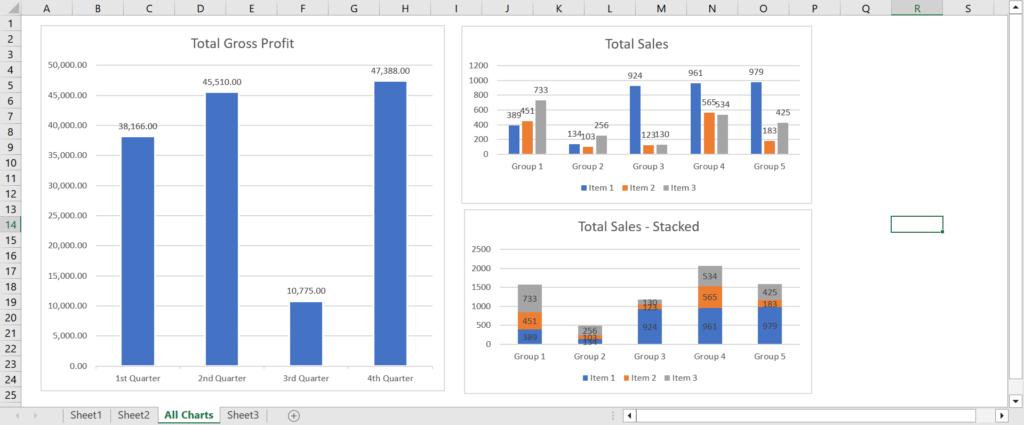
5. You should now see all the charts on top of each other in the “All Charts” worksheet (if you have not renamed it).
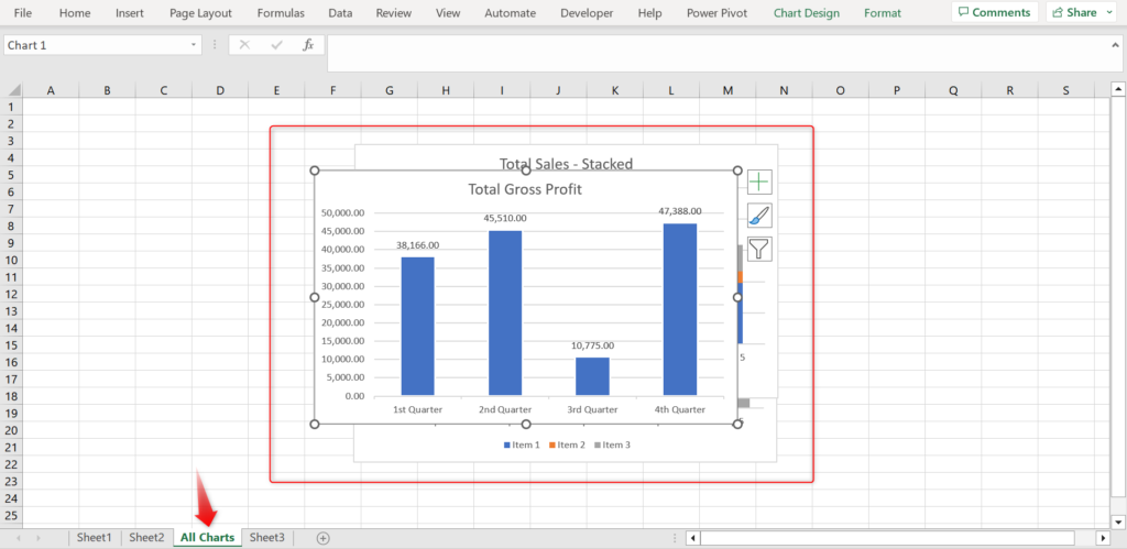
6. Click on each chart and drag them across the sheet to position them wherever you want them to be.

7. Also, as a pro tip, you might want to remove the gridlines from the worksheet to make it look clean, making the charts easier to read.
To do this, click the View tab from the Excel ribbon and uncheck the Gridlines checkbox under the Show section.

That’s it! All the gridlines should now disappear from your sheet.
8. When you close or save the file, you might encounter the following prompt:
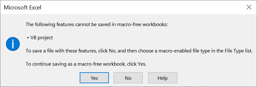
If you no longer need to run the code next time, click Yes to continue. Doing so will remove the macro from your file.
On the other hand, if you want to save the file with the code, click No and select .xlsm or .xlsb as the file format.
Conclusion
Excel charts are perfect for summarizing long rows of data. They give our targeted audience a glimpse of “what’s happening” through these graphical representations.
Organizing these charts and placing them on specific sheets can significantly increase the professional appeal of your workbook. I hope the suggested methods above help you do so with ease.