How to Remove Blank Rows in Excel?

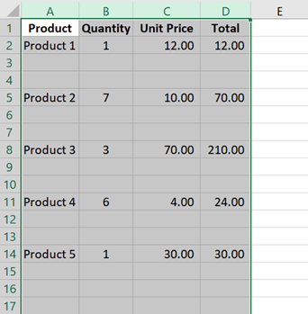
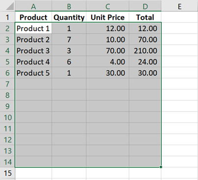
Blank or empty rows in between a dataset can be cumbersome to look at and work on.

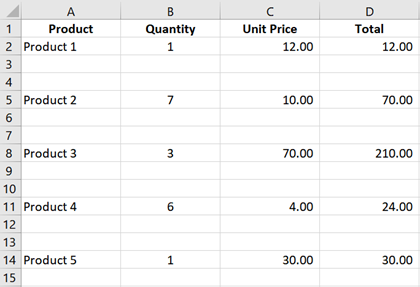
We often encounter this type of format with datasets exported from a system or a database.

With the blank rows in between, it’s hard to go over the data as you are forced to scroll down just to see the remaining data entries.

You can’t even select all the data by pressing CTRL + A.

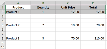
Example of what happens when you press CTRL + A to select all cells in the dataset

(Notice that Excel can only select the data entries before the blank rows.)

Also, if you try to apply the filter after selecting the headers, Excel is not able to capture all the records in the dataset (as seen in the example below).

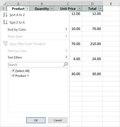
Exmple of what happens when you apply filter after selecting the headers in a dataset with blank or empty rows.

If you want the filter to work correctly with this format, you will have to either select the entire columns or manually select all the records in the dataset – which can be very inconvenient.

In this tutorial, I’ll show you different ways to remove these empty rows so you can easily work on your data.

Use the “Go to Special” option to Remove Blank or Empty Rows in Excel

The first step to removing blank or empty rows is to select the entire dataset.

Since we can’t make use of CTRL + A to select it, we can do either of the following:

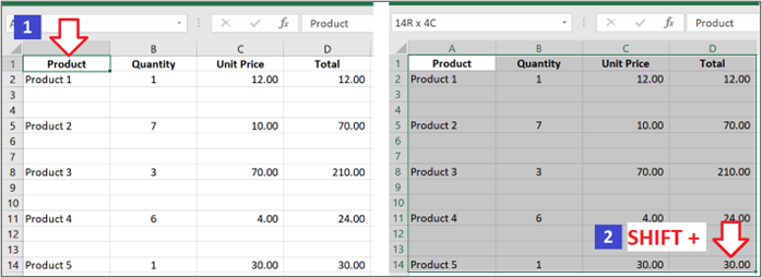
a) Select the entire columns of the dataset (as shown below).

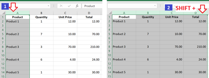
b) Or select the first cell and scroll down until you find the last cell of the data set. Then, while pressing the SHIFT key, click on it.

If you don’t have other data at the bottom of the data set, you may want to use the first option since that is the quickest way to select the cells.

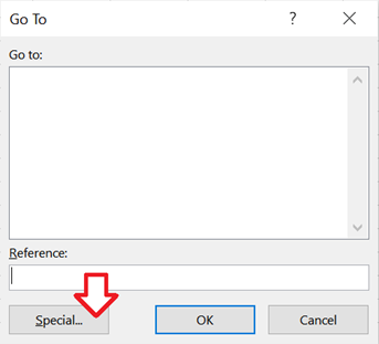
After highlighting the cells, press CTRL + G.

The “Go To” menu should appear. Once you see it, click on the Special… button.

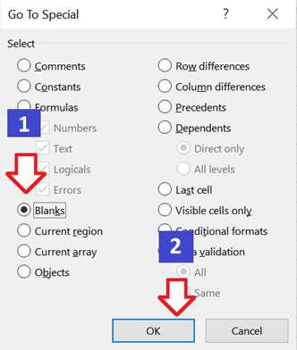
Click on the "Special" button from the "Go To" menu.

You will then see the Go To Special menu. Select Blanks and click OK.

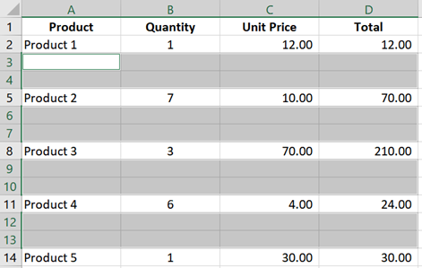
Steps to select blank cells from the "Go To Special" menu

Notice that the blank or null cells are highlighted.

Example of what happens when blank or null cells are highlighted

Right-click on one of these highlighted cells and select Delete.

Right-click on one of the highlighted cells and select Delete.

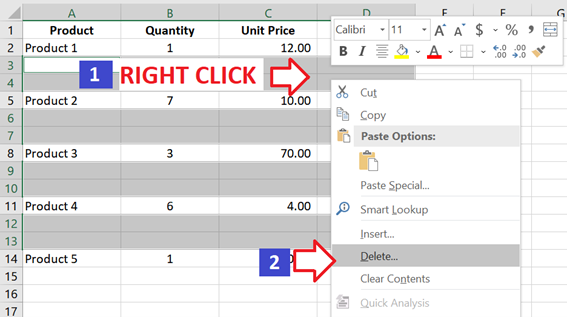
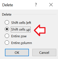
The Delete menu will appear. Select Shift cells up and press OK.

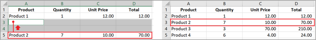
Select "Shift cells up" from the "Delete" menu and click OK.

And voila! You have now removed the blank rows from your dataset.

Note This

Remember to select the Shift cells up option (not Shift cells left).

This step is crucial to ensure that the remaining cells within your data move up after deleting the blank rows.

Example of what happens when you select "Delete Shift Cells Up"

If you select the Shift cells left option, the cells on the right will move towards your dataset.

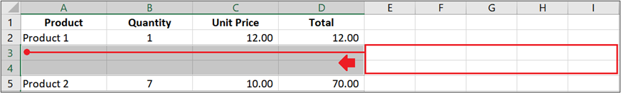
Example of what happens when you select "Delete Shift Cells Left"

If the cells on the right don’t have any contents (same as the image above), it will look like nothing is happening in the data set. However, if you have other datasets on the right side of your sheet, the datasets will all be mixed up.

You can use the Shift cells left option if you’re trying to delete columns in between the data set.

Using the Auto Filter to Remove Blank or Empty Rows in Excel

Another way to remove blank or empty rows is to use the Auto Filter. We will copy the dataset to a different sheet or workbook. If that’s not a problem, then this would be a good option too.

Select first the cells within the data set.

Same as the steps specified above, you can either:

Select the entire columns of the data set; or
Select the first cell up to the last cell within the data set.

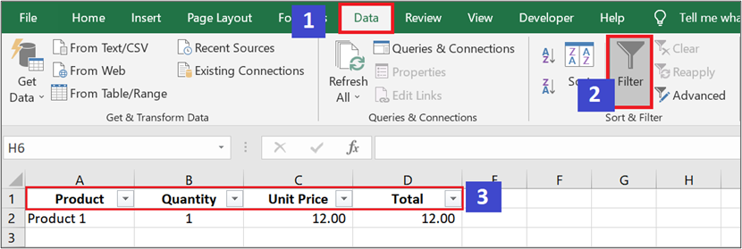
Once the cells are highlighted, apply the filters by going to the Data menu and selecting Filter.

You should then see the filters added to the header row.

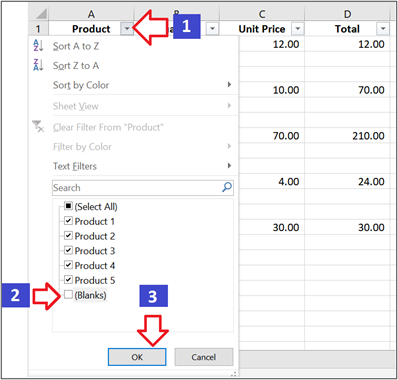
Steps to add filter to dataset with blank rows

Once the filters are in place, add a filter so that the blank rows are excluded from the data set.

To do this:

Select the filter in one of the fields.
Uncheck (Blanks) – this will be the last item in the filters.
Click OK.

Select the filter in one of the fields, uncheck "(Blanks)" and click OK.

You will now see the data set without the blank rows in between.

Once you see this, copy the filtered data set (CTRL + C) and paste it (CTRL + V) on a different sheet or workbook.

Using the FILTER() Function to Remove Blank or Empty Rows in Excel

This method is probably my favorite as it involves the least number of steps.

IMPORTANT:

FILTER() is a dynamic array function that only works on Office 365. If you’re using other versions of Office, I’m sorry, but this won’t work for you.

The FILTER() function uses the following syntax: =FILTER(Array, Include, [Empty])

“Array”is the data range to apply the filter to.
“Include” is the logical expression to use to filter the data.
“Empty” is the text you would like to appear if there are no results to display after applying the filter. This field is optional and can be left blank.

On a new worksheet (or on an empty section in the current worksheet), select a cell and type the FILTER() formula.

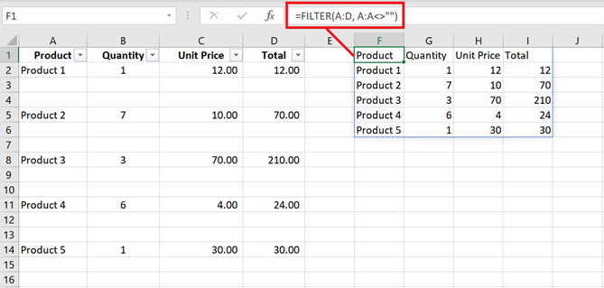
Add the FILTER() formula to one of the cells.

In my example above, I have used this formula: =FILTER(A:D,A:A<>””)

Change “A:D” with the range address where your dataset is located.
Change“A:A” with a column that can be used for filtering out blank rows.

And that’s it! As you press enter, you will immediately see your dataset without the empty rows.

What’s so cool about this is that if there are new entries added to the specified range, they will be immediately reflected in the filtered dataset.

Sorting the Records to Remove Blank or Empty Rows in Excel

If the previous method didn’t work for you, there’s still an easy way to remove the empty rows with just a few steps.

IMPORTANT: This method requires reordering your dataset. If this is not an issue, please proceed.

1. Select the entire column (or all cells within your dataset).

2. Go to the Data tab and click on the Sort button inside the Sort & Filter section.

3. In the Sort menu, select the field that we will use as the basis for sorting the records (it can be any field).

In the Sort menu, select the field to use as the basis for sorting the records (it can be any field).

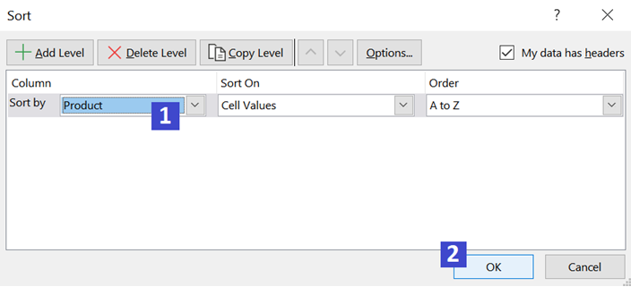
You can also change the sort order to either ascending or descending order – it doesn’t matter.

Once done, click OK.

And that’s it! Blank rows will “disappear” from your dataset.

Using Power Query to Remove Blank or Empty Rows in Excel

As mentioned, we mainly get empty rows from files exported from a system or a database.

If you regularly receive these kinds of files and would prefer to have the empty rows automatically removed, then this next method is for you.

1. Set up a Power Query to load the file.

(If you have an existing Power Query already set up on your data, you can skip this step and add the rule specified in step #4.)

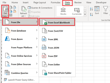
On a new workbook, go to Data >> Get Data >> From File >> From Excel Workbook.

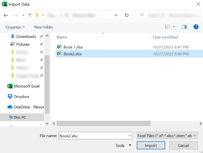
2. The Import Data menu will appear. Select the file that contains your dataset and click Import.

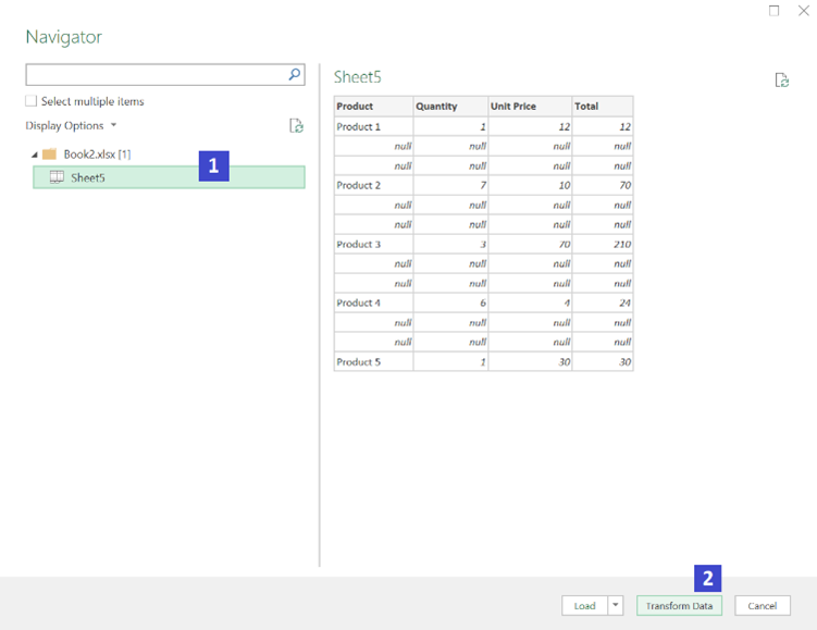
Select the file to import from the "Import Data" menu of the Power Query.

3. In the Navigator menu, select the sheet that contains your dataset and click on the Transform Data button.

4. Wait for the data to load.

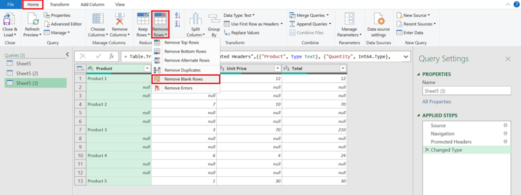
Once the Power Query Editor appears, click on Remove Rows >> Remove Blank Rows.

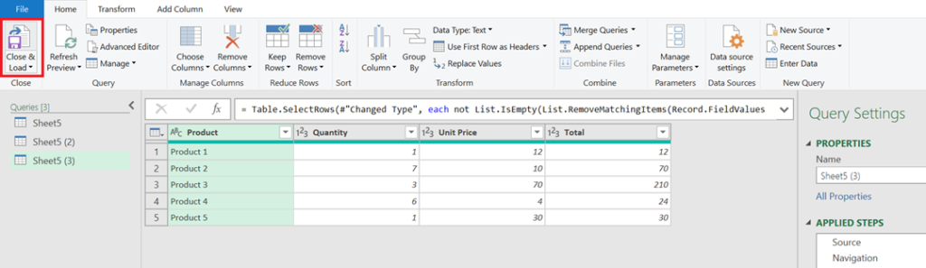
5. You will see the empty rows filtered out from your dataset.

Once you see that, click on the Close & Load button.

Once you see the empty rows filtered out from your dataset, click on the "Close & Load" button.

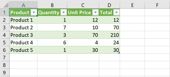
And that’s it! Your Power Query Table is all set up.

Sample output after removing blank rows using Power Query

If you receive a new export file, place it in the same folder as the current file and replace the existing one. Make sure that the filename is the same.

Then, open the workbook with the Power Query Table, right-click on the table and select Refresh to get the latest set of data. The Power Query will automatically remove the empty rows from the dataset.

Conclusion

Blank or empty rows within a dataset are at times inevitable especially if you’re working on an exported file. I hope with the methods suggested above, you will find it easy to remove these unnecessary rows from your dataset.