A comma (,) is a tool that we use to separate words in a text or digits in a number so that we can better read and understand them at one glance. There are, however, instances when we need to remove them from our dataset.
In this tutorial, I will show you different ways to remove the comma from a number and text in Excel.
Remove Commas from a Number in Excel
When removing commas from a number in Excel, the first step is to determine whether the commas are part of the value inside the cell or they were only added as part of the cell formatting.
To determine which reason applies to your cell, you only need to:
- Click on the cell that contains the number.
- Look at the formula bar and see if you can find a comma in there.
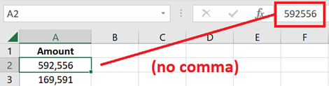
If you cannot find the comma, it means that the comma is part of the cell’s number formatting; therefore, you need to change the number formatting to remove it.
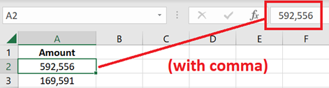
If you see the comma, it means that the cell, even though it contains a number, is being treated by Excel as text.
Remove Commas from a Number by Changing the Number Format
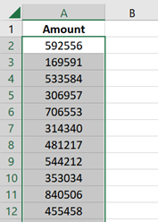
1. Highlight all the cells containing numbers with commas.
2. Go to the Home tab and click on the small arrow on the rightmost side of the Number section.
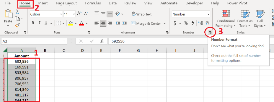
The Format Cells menu should appear.
If you like keyboard shortcuts, you can press CTRL + 1 to do this.
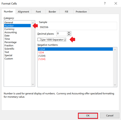
3. You have two options to remove the comma:
You can set the format to General and click OK.
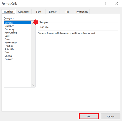
Or you can set it to Number, uncheck the ‘User 1000 separator (,)’ option, and click OK.
4. And that’s it! Commas are now removed from the numbers inside your selected cells.
Remove Commas from a Number in Text Format
If you see the comma in the Formula Bar whenever you click on the cell, it means it was added as part of the value. Even though the cell contains a numeric value, Excel sees it as text, which means you can’t use it in calculations.
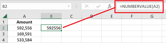
To remove the comma, we will have to retrieve the numeric value using the NumberValue() function.
On a new column, type the following formula: =NUMBERVALUE(A2)
Change “A2” with the appropriate range address of your cell.
And that’s it! You have successfully extracted the numeric value from the selected cells.
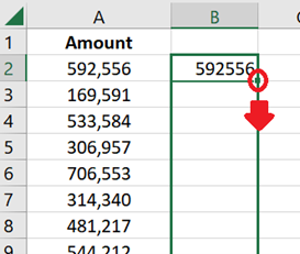
Copy this formula to the remaining cells by dragging the Fill Handler down, and you’re all set.
NOTE: If you still see the comma after entering the formula, update the cells’ number formatting (as described in the previous method).
Remove Commas from a Text in Excel Using Find and Replace
1. Highlight all the cells where you would like to remove the comma.
2. Go to the Home tab. Under the Editing section, click on Find & Replace >> Replace.
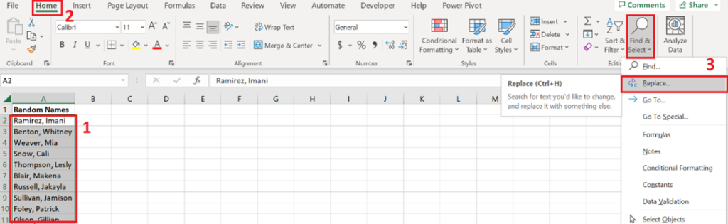
The Find and Replace menu will appear.
If you like keyboard shortcuts, you can simply press CTRL + H.
3. In the Find What textbox, type a comma. Leave the Replace With textbox blank and click on the Replace All button.
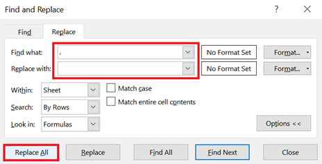
And voila! All commas will disappear from the selected cells.

Remove Commas from a Text in Excel Using the SUBSTITUTE() Function
This method is perfect for those who don’t want to modify the dataset and prefer to have a new column store the texts without the commas.
Also, you’ll have the option NOT to remove all the commas inside the cell. You can freely select which comma to remove. Pretty sweet, right?
The SUBSTITUTE() function allows us to replace one or more text strings with a different text string.
=SUBSTITUTE(text, old_text, new_text, [instance_num])- text refers to the range containing the text that you would like to remove the comma from.
- old_text refers to the text that you would like to replace which, in this case, is the comma.
- new_text refers to the replacement of the old text. Since our goal is to remove the commas, we will set this to blank.
- [instance_num] is optional. Leave this blank if you want to remove all instances of commas inside the text. However, if you only want to remove one of the commas inside the text, use this parameter to specify which instance of the comma to remove. (e.g., 1 for the first, 2 for the second)
You can copy either of these formulas:
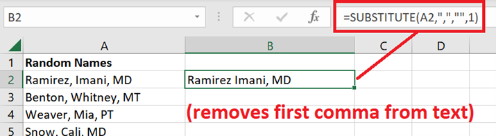
| =SUBSTITUTE(A2,”,”,””) | This removes all instances of the comma inside the text. |
| =SUBSTITUTE(A2,”,”,””,1) | This removes the first instance of the comma. |
Change “A2” with the appropriate range address of your cell.
If applicable, change “1” with the instance of the comma that you would like to remove.
Copy this formula to the remaining cells, and you’re all set.
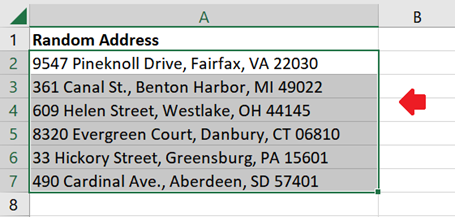
Remove Commas from a Text in Excel and Separate Data in Different Columns
This method will not only remove the comma from the text but will also split the data and place them each in separate columns.
1. Highlight all cells that you would like to split into multiple columns.
IMPORTANT:
Since this method will split your data into multiple columns, the columns next to the selected cells should be empty and have no data.
You could temporarily copy the cells on a different sheet and just copy them back later into your dataset.
2. Go to the Data tab. From the Data Tools section, click on Text to Columns.

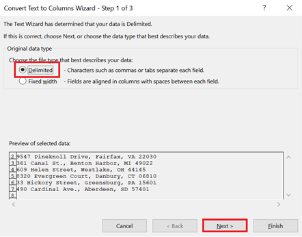
The Convert Text to Columns Wizard will appear.
3. Select the Delimited option and click Next.
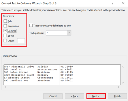
4. From the list of Delimiters, ensure that only the Comma checkbox is checked and click Next.
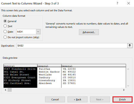
5. In the last step of the Wizard, you can configure the data format for each column.
But we will skip this step and leave the default format for now. You can update the number format of the columns later.
Let’s complete the Wizard and click on the Finish button.
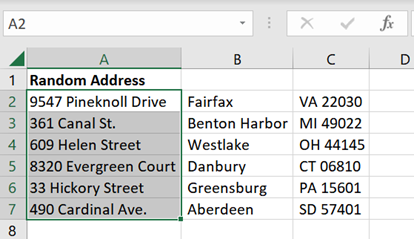
6. And that’s it! Your data is now split into multiple columns.
Conclusion
As you can see, the approach we use to remove the commas in our cells will depend on the type of data we have on our cells (whether it’s a text or a number). It also depends on whether we would like the data to be split into multiple columns or not.
Whatever your intended purpose may be, I hope you find the suggested methods helpful.