Splitting a worksheet into panes or sections is great for keeping certain contents within the sheet (like the headers) to be always on display even when we scroll to other areas in the sheet.
Excel allows us to split the worksheet into two or four panes. Once a worksheet is split, you can scroll through each section independently.
There are times, however, when we need to remove these panes so we could view the worksheet again as a whole and do other things within the sheet.
There are four simple ways to do these.
Table of Contents
1. Double Clicking on the Dividing Bar
If you have four panes added to your worksheet and want to remove just one of the panes, all you need to do is double-click on the dividing bar that you want to remove.
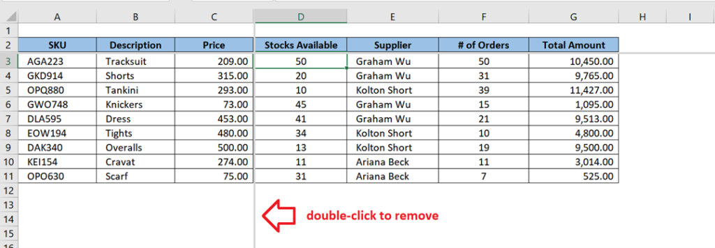
That’s it! You have a single pane removed.
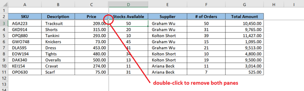
On the other hand, if you want to remove all the panes at once, double-click on the intersection between the dividing bars.
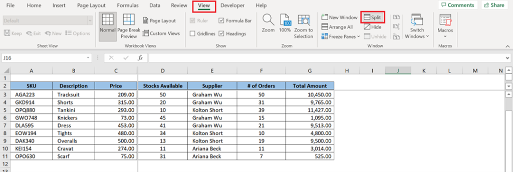
2. Clicking on the “Split” button
Another quick method to remove all panes at once is by going to the View menu and clicking on the Split button.
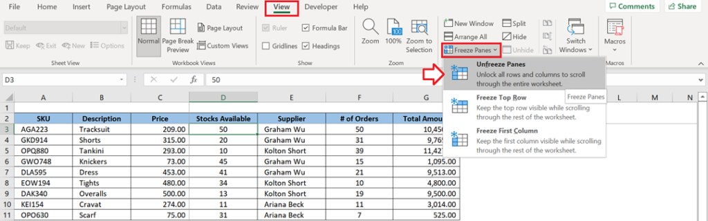
3. Unfreezing the Panes
If you have added panes in your worksheet by freezing the rows and/or columns, you can easily remove the panes by going to the View menu.
From the Windows section, click on Freeze Panes and select Unfreeze Panes.
4. The Keyboard Shortcut
For keyboard warriors out there, the fastest way to remove the panes is by pressing ALT + W + S.
Related Tutorial: How to Remove Dashes in Excel
Conclusion
Splitting a worksheet into panes is a huge help whenever we need to compare the values in different areas of the worksheet. There are, however, instances when we need to view the worksheet again as a whole. As you have seen in the examples above, with just a few clicks or keyboard entries, you can easily remove these worksheet panes.