How to Select Alternate Rows in Excel? (or Every Nth Row)

There are plenty of possible reasons we need to select alternate or every nth row in Excel.

It could be:

• To change these rows’ cell formatting or color to highlight them and make the dataset more readable.
• To delete the contents of these rows. (Note: we have a separate article for this. You may also want to check out “How to delete every other row“.)
• To copy and paste them on a different sheet.

Whatever your reason may be, I will show you quick and easy ways to select every odd, even, or nth row in Excel.

Note that each method is designed to achieve a particular task. Some may be useful for highlighting rows. Others are useful for filtering the dataset so you can readily transfer every nth row to somewhere else. 

I suggest you go over each method, so you will have something to use in the future in case you need it.

Highlight Alternate Rows by Formatting the Data as Table

The quickest way to highlight alternate rows in Excel is to format your dataset as a table. To do this:

1. Select your entire dataset.

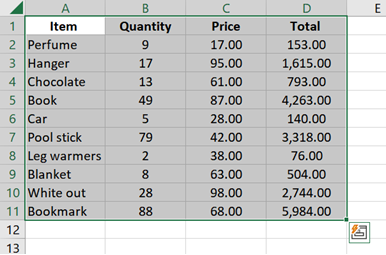
You can do so by clicking on one cell from your dataset and pressing CTRL + A.

2. Once the entire dataset is selected, press CTRL + T. This will trigger Excel to convert the selected cells into a table.

You will see the Create Table menu pop up. The range that you have selected will appear in it.

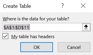
If your range has headers, tick the “My table has headers” checkbox. Otherwise, untick the checkbox.

Once done, click OK.

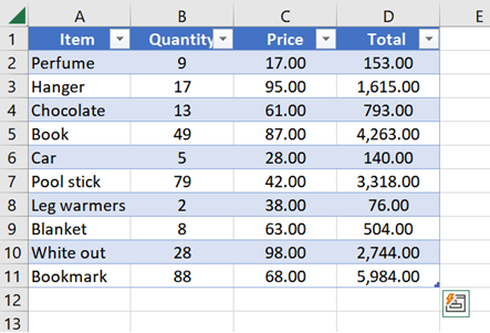
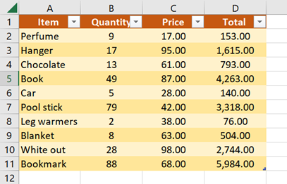
3. And that’s it! You have converted your data range into a table with alternate row colors. 

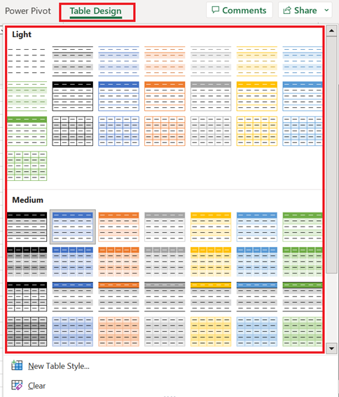
4. If you like, you can change the color of the alternate rows in your table. With the table selected, go to the Table Design tab.

You can select from the preformatted table designs.

You can also be creative and create your very own table design. All you need to do is click on the New Table Style option at the bottom of the Table Designs.

The New Table Style menu will appear.

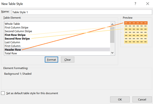
Choose a table element and click the Format button to change its format.

In my example above, I have updated the following table elements:

• First Row Stripe (odd rows in your dataset)
• Second Row Stripe (even rows in your dataset)
• Header Row

Once you have configured all the desired elements, click OK.

Go back to the list of table designs and select your custom design.

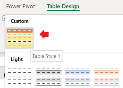
And that’s it! You now have your dataset with the alternate rows highlighted.

Highlight Alternate or Every Nth Row Using Conditional Formatting

This method is perfect for those who don’t want to convert their data into a table. It allows you to specify which nth row needs to be highlighted. It doesn’t necessarily have to be the odd or even rows. It could be every 3^rd, 4^th, 5^th, or whatever row in your dataset.

1. Select all cells in your dataset except for the header.

2. From the Home tab, go to the Styles section and click on Conditional Formatting >> New Rule.

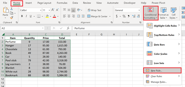
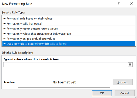
3. The New Formatting Rule menu will appear.

From the list of Rule Types, select “Use a formula to determine which cells to format”.

4. Now, it’s time to define the formula that will serve as the basis for highlighting a particular row.

You can choose from the following formulas:

• =ISEVEN(ROW())=TRUE
  • Use this to highlight all even rows.

• =ISODD(ROW())=TRUE
  • Use this to highlight all odd rows.

• =MOD(ROW()-[header row], [nth row])=0
  • Use this to highlight every nth row.
  • [header row] refers to the row where your header row is. If it’s in row 1, then type 1. Set this to 0 if your dataset doesn’t have a header.
  • [nth row] refers to the nth row in the dataset you would like to highlight. So, if you’d like to highlight every 3^rd row in your dataset, set this to 3.

5. Once you have identified your formula, type it in the “Format values where this formula is true” textbox.

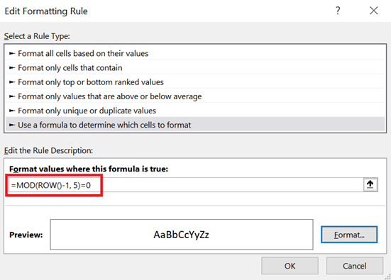
In my example above, I have used this formula: =MOD(ROW()-1,5)=0

Notice that my header is in row 1. My target is to highlight every 5^th row in my dataset.

6. After adding your formula, click the Format button to select the color you want to highlight these rows.

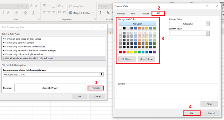
The Format Cells menu will appear. Go to the Fill Tab and select your desired background color. Once selected, click OK.

7. You will be redirected back to the previous menu where you’ll see a preview of the format you selected.

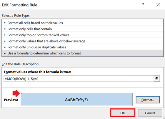
If you want to change it, click the Format button again. But if you’re already happy with it, click OK.

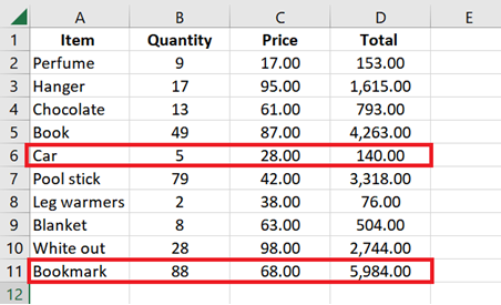
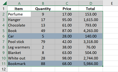
8. And that’s it! You should now have every nth row in your dataset highlighted.

Select Alternate or Every Nth Row in Excel Using the “Go to Special” Method

This method is perfect for any kind of purpose. You can use this to color every nth row, copy them into a different sheet, insert the same text to every other row, delete every other row, etc.

For this method, we will add a formula that will mark the rows we intend to select.

You can use either of these formulas:

• =ISEVEN(ROW())
  • Use this to select all even rows.

• =ISODD(ROW())
  • Use this to select all odd rows.

• =MOD(ROW()-[header row], [nth row])=0
  • Use this to select every nth row.
  • [header row] refers to the row where your header row is. If it’s in row 1, then type 1. Set this to 0 if your dataset doesn’t have a header.
  • [nth row] refers to the nth row in the dataset you would like to select. So, if you’d like to select every 3^rd row in your dataset, set this to 3.

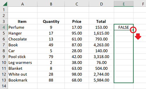
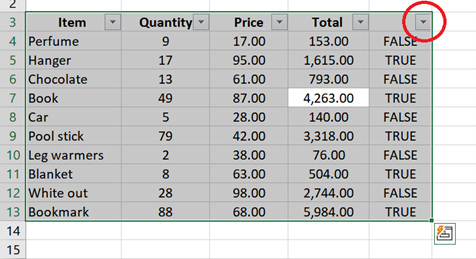
1. On a new column next to your dataset, type the formula that you have chosen to use.

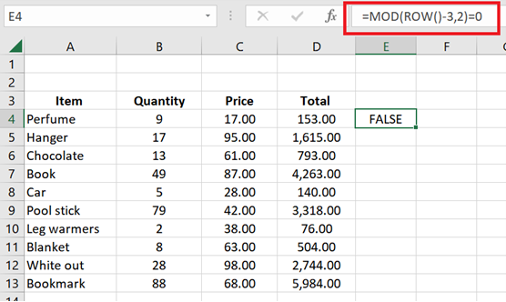
In my example above, I used this formula: =MOD(ROW()-3, 2)=0

Notice that my header is in row 3. I wanted to select every 2^nd row in my dataset.

2. After adding the formula, drag the Fill Handler down until the last row in your dataset to copy the formula to these cells.

3. Our goal is to mark all rows that we intend to select with TRUE.

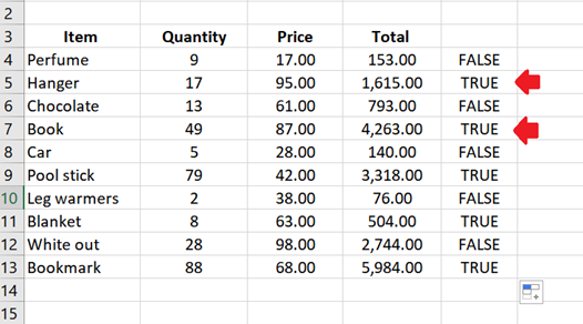
Check the first few rows in your dataset and see if you have achieved this goal.

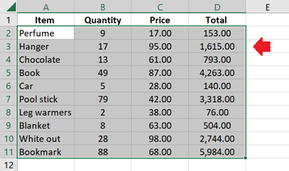
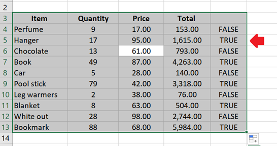
4. Once you’re satisfied with the result, select all the cells in your dataset.

You can do so by selecting one cell within the dataset and pressing CTRL + A to select all.

5. From the Data tab, go to the Sort & Filter section and click on the Filter button. 

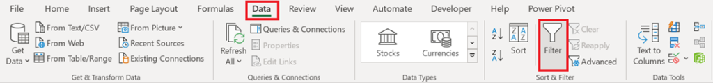
6. Filters will be added to your dataset.

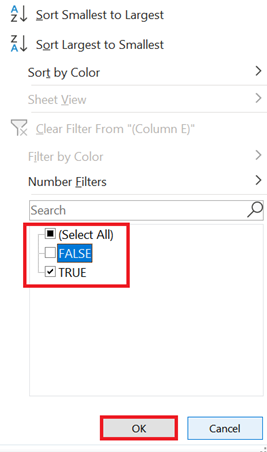
7. Click the filter on the column we have added. Untick the FALSE checkbox and click OK.

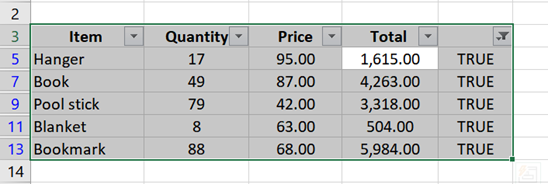
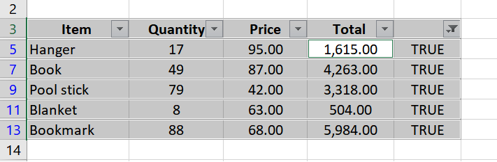
8. Your dataset will then be filtered to only show rows marked as TRUE.

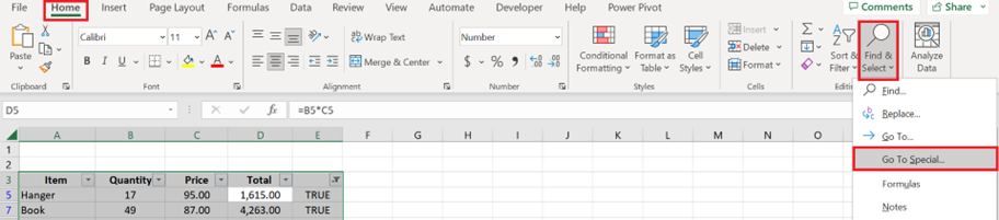
9. While all the cells in the dataset are selected, go to the Home tab.

From the Editing section, click on Find & Select >> Go To Special.

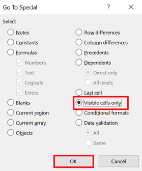
10. In the Go To Special menu, select Visible cells only and click OK.

11. And that’s it! Every nth row in your dataset is now individually selected.

12. You can now do whatever you want with these cells.

You can change the cell formatting or the cell colors to highlight them.

If you want to copy them to other cells, you can do so by pressing CTRL + C to copy.

If you want to delete them, right-click on one of the cells and select Delete Row.

Conclusion

As you can see, there are plenty of ways to select alternate or every nth row in Excel. The first two methods show you the quickest ways to highlight rows. The last method, on the other hand, is perfect for all selection purposes.

Check our related tutorial about removing the header or footer in your sheet.