Peeking a little back to high-school times, we all have had a tough time learning tricks to square a number as quickly as possible. Manual squaring can often turn out super challenging, particularly when dealing with a large value or a large set of data.
With excel, you can square a number instantly without having to put together too much effort. To learn all about squaring a number or a list of numbers in excel, continue reading.
How to Square a Number in Excel?
There are four common ways how you can end up squaring a number in excel. Let’s look into each of them below.
1. Using the Multiplication Formula to Square a Number in Excel
Putting together a formula in excel gets pretty interesting once you understand how excel works. Here is how you can compose a quick formula to yield the square of a number in excel.
Select the cell where you want the square of the number to be populated and type in the following formula.
=Cell Reference * Cell Reference
Here cell reference represents the cell that contains the number to be squared. Here is how you may bring this formula to action.
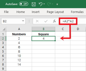
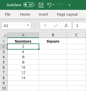
In the screenshot above, A2 contains the number to be squared, and therefore, the formula is accordingly amended as :
=A2*A2
The value in B2 represents the square of the value in A2 i.e. 2. It is only this easy – to apply the same formula to an entire list of numbers, capture the fill-handle button and drag it down till needed.
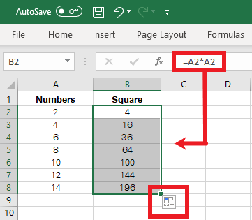
If you already have the list ready in either of the neighboring columns/rows, simply double-click the Fill-Handle icon to have the square list populated automatically. Here is how excel auto-fills the square of the given numbers.
2. Using the Caret Formula to Square a Number in Excel
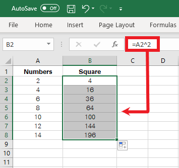
Another simple and quick way to yield the square of a number is using the caret (^). A caret in excel is used to represent exponential power. As square represents the power ‘2’, using caret with the power 2 gives back square of the base value.
Let’s stipulate it below. Activate a cell to input the following formula.
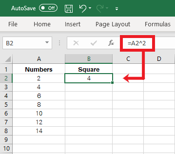
=A2 ^ 2
Here cell A2 contains the number that is to be squared. Excel gives the following results.
Drag down the Fill Handle to have the same applied to a list of numbers.
3. Using the Power Function to Square a Number in Excel
The power function of excel works to raise a number to a certain power. The syntax of the power function looks as follows.
= POWER (number, power)
- Number represents the number that is to be squared
- Power represents the exponential power to which the number is to be raised
Let’s put together an example to see how this function works.
In the data given below, to find the square of the numbers given in Column A, the power function is to be applied as below.
=POWER (A2, 2)
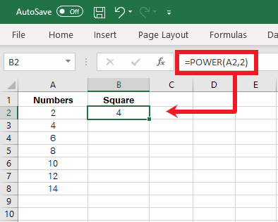
Cell A2 contains the number to be squared. A number is squared when raised to the exponential power 2 so the power is set as 2.
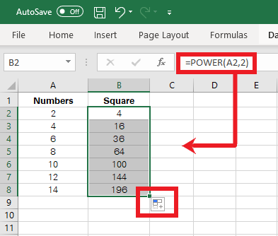
Next, just drag the Fill Handle to find the square of all the numbers appearing in Column A.
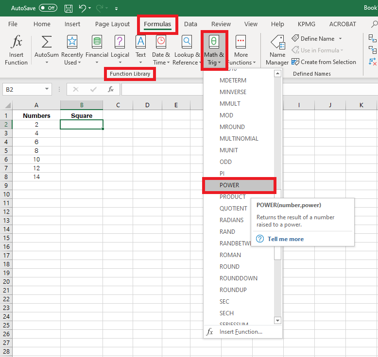
Pro Tip: No need to cram the Power function. Find it out in the Function library by going to the Formulas tab > Function Library > Math & Trigonometry > Power Function
4. Using the PRODUCT Function to Square a Number in Excel
This method is very similar to the multiplication formula. However, using this method, you can employ an Excel function to yield the square of a given number.
The Product function of excel purports to find the product of two, three, or more numbers. All the numbers fed within the formula act as arguments and must be separated by commas to be recognized by Excel.
The syntax of the Product function reads as follows:
=PRODUCT (Number 1, Number 2)
In the above formula number 1 and 2 represent the two numbers to be multiplied. These can be numeric values or cell references.
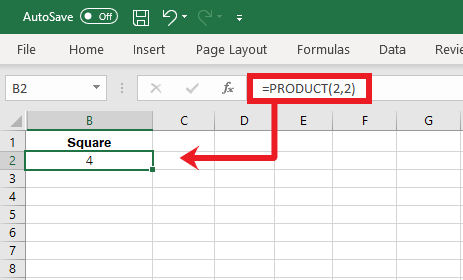
For example, to use the above formula with numeric values to find the square of ‘2’, you may amend it as follows.
=PRODUCT (2, 2)
Excel would yield the square of 2 as evident in the screenshot below.
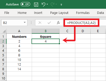
To use the PRODUCT function to find a square with cell references, you may amend it as follows:
=PRODUCT (A2, A2)
Excel would yield the square of the value contained in cell A2 as evident through the screenshot below.
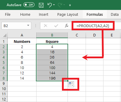
When using the PRODUCT function with a cell reference, you can auto-fill the formula for a list of cells by simply dragging the fill handle. Here is how it works.
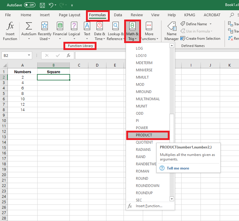
Pro Tip: Find the Product function the Functions Library by accessing the Formulas tab > Function Library > Math & Trigonometry > Product Function
Conclusion:
Finding the square of a number is an exercise that you’ll come across every so often. But once you’ve picked up on the above-explained easy methods to find the square of a number, it should no more concern you.
No matter how lengthy the figure gets, using either of these methods would help you track down the square of any number with accuracy and precision. And if the list of numbers keeps going on, let the fill handle do the job. Hope this article helped you learn and grow!
Suggested Tutorial: How to Remove Hyperlink in Excel?