Before anything, what is a stem and leaf plot? You are likely to not have heard of it before. However, the general idea that first hits your mind upon hearing of a stem and leaf plot is a plot that might have many leaves rooting from a stem.
That’s exactly how a stem and leaf plot is. Under a stem and leaf plot, we break each number of a given data set into a stem and leaf.
To keep you short on surprise, here is how the idea of a stem and leaf plot looks in action.
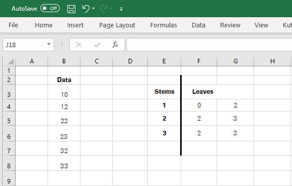
Clearly visible above, the first digit of every number serves as the stem and the last digit makes it up like a leaf.
A stem and leaf plot visualizes the distribution of numbers within a range. These plots are helpful as they allow users to perform a quick analysis of the distribution of data across different categories.
Not only does it help you with easy scanning of data, but also with the calculation of mean, median, mode, and other statistical basics.
Creating a Stem and Leaf Chart in Excel
We have seen Excel put together bar charts, line charts, pie charts, scatterplots and so many more. But when it comes to a stem and leaf plot, Excel doesn’t offer an in-built function for creating a stem and leaf plot.
However, that must not stop you from building a stem and leaf plot in Excel through alternate methods. For now, let us look into the most basic method for creating a stem and leaf plot in Excel.
It is to be noted that this method is manually driven and works best for sets of smaller sizes (under 100s).
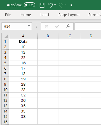
To create a stem and leaf plot from the above data series, the following steps are to be followed:
Step 1:
First of all, the data must be arranged in ascending order for ease of plotting. To do so, select the data and go to:
Home Tab > Editing > Sort & Filter > Smallest to Largest
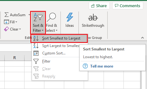
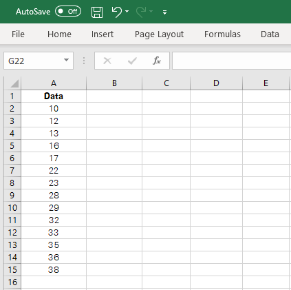
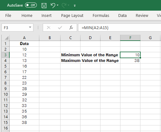
Excel will arrange the data in ascending order as shown below.
Step 2:
Determine the minimum and maximum values of your data set to plot the stems. This can be done through the Minimum and Maximum functions as shown below.
Step 3:
With 10 and 38 as the minimum and maximum values, we know the data lies between 10s to 30s. The stems, therefore, range from 1 to 3 (the first digit of 10, 20, and 30).
Plot the said range in a column as shown below.
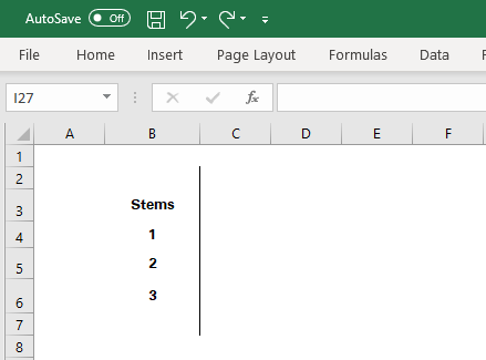
Pro Tip:

For better presentation, you may align the stems to the right and add a right side border to them. Unchecking the ‘Show Gridlines’ mode from View Tab > Show > Gridlines can add to the visual appeal of the plot.
Step 4:
The next step is to plot the leaves across the plot. There are two ways how this can be done.
- Manually, by tally-marking each number from the data and adding a leaf for each number against the relevant stem.
- Using the COUNTIF formula nested in the REPT Function which might get complex and super lengthy.
We have plotted the leaves in the plot manually by plotting the last number of each digit in a cell against the relevant stem (first digit of that number). The plotted chart should look like the following.
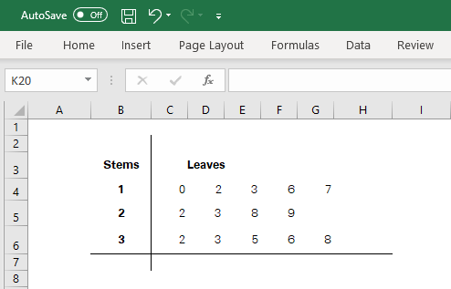
And that’s it! Your stem and leaf plot is all done.
Pro Tip: As this plot is only manually made, it is prone to human error. A quick way to check your stem and leaf plot for accuracy is to count the number of leaves. As our dataset consists of 14 numbers in total, there should be 14 leaves on the plot.
Bottom Line
We hope you enjoyed making a stem and leaf plot in Excel.
Must note that there can be many variations to the steps involved above and how the final plot looks like.
The methods discussed above are the most basic ones that will help you plot a small data set.
However, as the data grows in size, you might need to move to other methods.