When working with exported data, there will be times when we will have only the month and year included in the dataset (the day is nonexistent).
It was okay until you realized that, for very particular reasons, you must turn these two bits of information into an actual date.
In this tutorial, I will teach you how you could convert your month and year to an actual date. Also, in the latter part of this article, I will teach you how to do it in reverse – from date to month and year.
Table of Contents
Steps to convert month and year to date in Excel
Since I have no idea how your month and year are currently formatted, we have to do some data prep to ensure that we are working on the same data format.
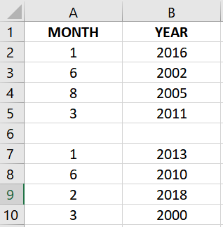
Our goal is to have our month and year look something like this:
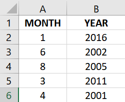
* The month is in numerical format (1 to 12).
* The month and year are on separate cells.
If your data already looks something like the image above, you can skip the following data prep sections.
IMPORTANT:
Before doing the data prep, please copy your Year and Month column to a new sheet and perform the data prep steps there. We want to ensure that your dataset is safe from accidental alterations.
Data Prep: Split Month and Year and place them on separate cells using the “Text to Columns” option
We have to split our Month and Year and place them in separate cells.
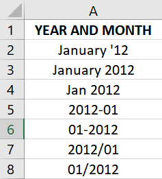
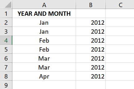
If they are joined together by a space, a dash (-), a slash (/), or any other symbol (similar to the image below), the fastest way to split them is by using the “Text to Columns” option.
To do this:
1. Highlight all the cells containing the year and month. Do not include the header.
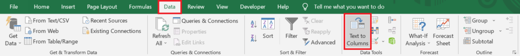
2. From the Data menu, click on Text to Columns.
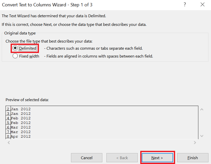
3. The Convert Text to Columns Wizard will appear. From the list of options, select Delimited. Then, click Next >.
4. Now, select the appropriate delimiter for your data.
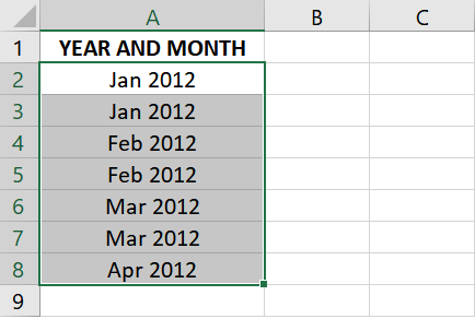
In my example, a space separates the month and year (e.g., Jan 2012).
Since this is the case, I have unchecked all other delimiters and only ticked the Space checkbox.
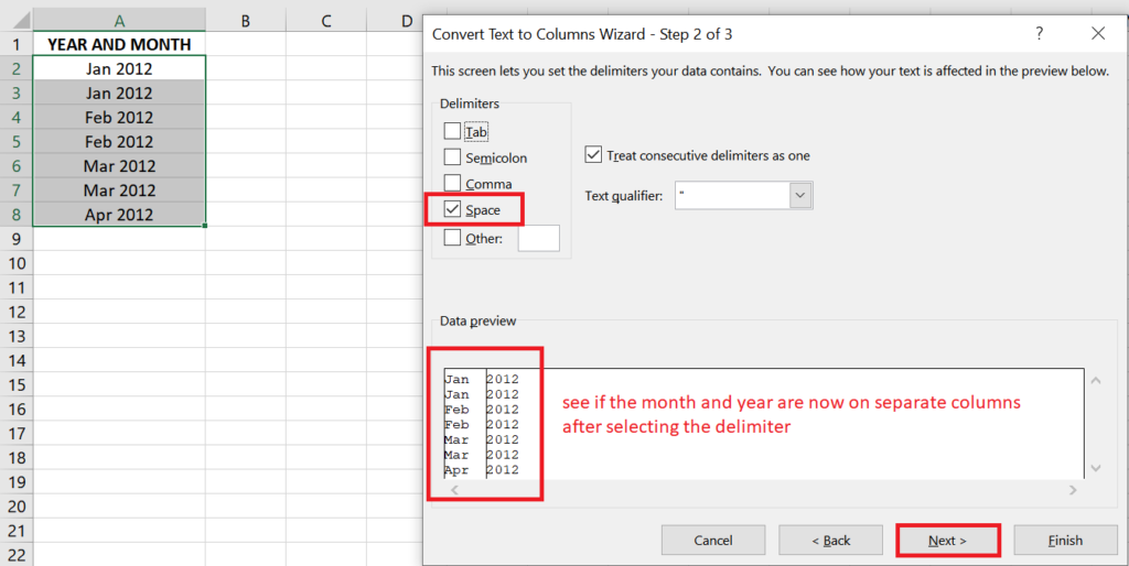
You know you have selected the correct delimiter once you see your month and year on separate columns in the Data preview.
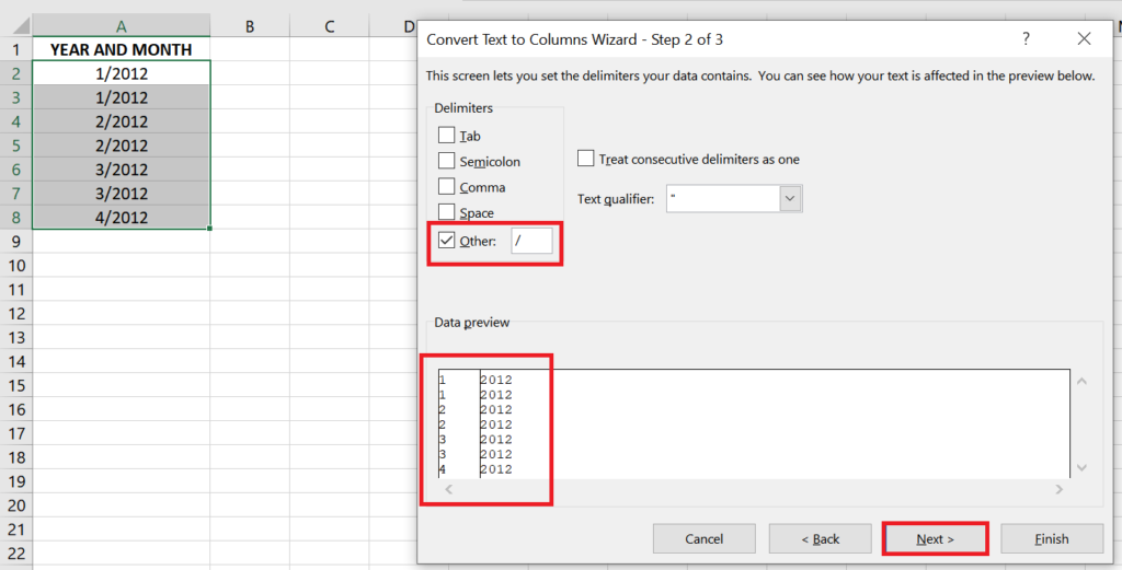
If your delimiter doesn’t exist in the list of available options, tick the Other checkbox and type the symbol that separates your month and year.
Once you’re happy with the result, click Next >.
5. You should now reach the final step in the Wizard.
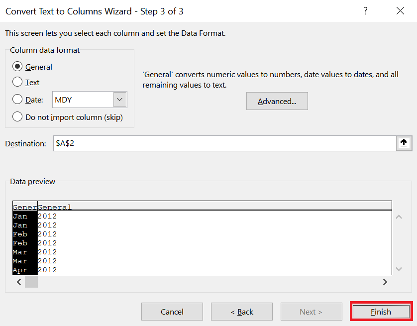
We are not going to change anything on this step. Just click the Finish button.
That’s it! You should now see your month and year in separate columns.
Data Prep: Split Month and Year and place them on separate cells using the LEFT() and RIGHT() Excel formulas
If your month and year are on a single cell but don’t have a space or any symbol in between them, we are to split them using Excel formulas.
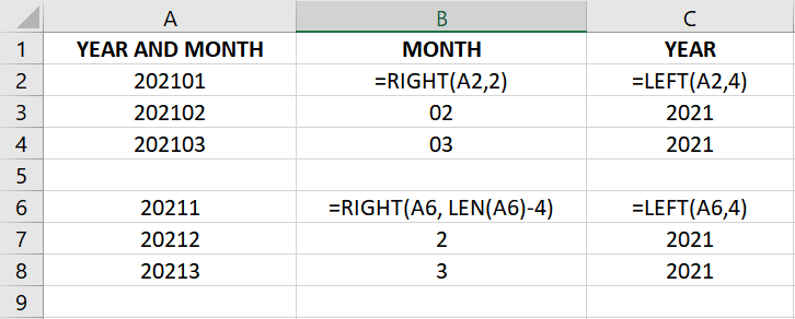
Below are some of the sample formulas that you can use. Note that the following formulas assume that your month and year are on cell A2.
| SAMPLE YEAR AND MONTH | FORMULA TO EXTRACT MONTH | FORMULA TO EXTRACT YEAR | NOTES |
| 201201 | =RIGHT(A2,2) | =LEFT(A2,4) | The year and the month have a fixed number of digits (4 and 2, respectively). |
| 20121 | =RIGHT(A2, LEN(A2)-4) | =LEFT(A2,4) | The year has a fixed number of digits (4), while the month has either 1 or 2. |
If your month comes before your year, you only need to swap the LEFT() and RIGHT() functions and adjust the character length accordingly.
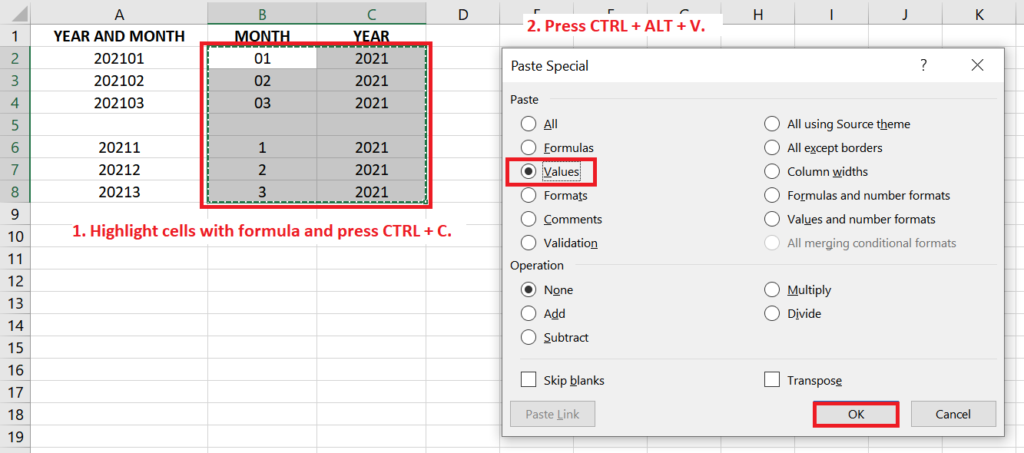
Once you’ve added the appropriate formulas, copy them and paste them as values.
To do this, highlight all cells containing formulas and press CTRL + C. Once the cells are enclosed with broken lines, press CTRL + ALT + V. From the Paste Special menu, select Values, and click OK.
Data Prep: Convert the Month in Text Format (e.g., February or Feb) to Numerical Format (e.g., 2)
Now that we have the month and year in separate columns, we move on to the last step for Data Prep.
You may skip this step if your month is already in numerical format (1 to 12).
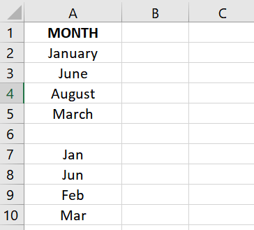
But if it is in text format (e.g., February, Feb), please follow these steps:
1. Insert a new sheet.
2. Copy your Month column and paste it into column A of the new sheet.
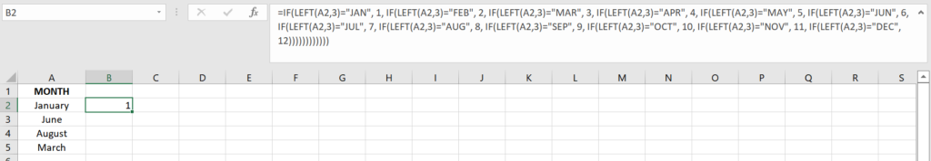
3. On cell B2, add the following formula:
=IF(LEFT(A2,3)="JAN", 1, IF(LEFT(A2,3)="FEB", 2, IF(LEFT(A2,3)="MAR", 3, IF(LEFT(A2,3)="APR", 4, IF(LEFT(A2,3)="MAY", 5, IF(LEFT(A2,3)="JUN", 6, IF(LEFT(A2,3)="JUL", 7, IF(LEFT(A2,3)="AUG", 8, IF(LEFT(A2,3)="SEP", 9, IF(LEFT(A2,3)="OCT", 10, IF(LEFT(A2,3)="NOV", 11, IF(LEFT(A2,3)="DEC", 12))))))))))))
This formula will get the numerical value of the month.
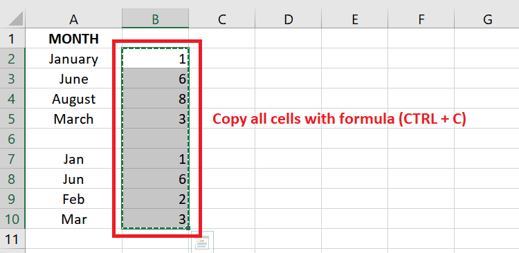
4. Copy cell B2 and paste it onto the remaining rows.
5. You should now see the corresponding numerical values of your months.
6. Once you’re happy with the result, highlight all the cells with formulas in column B and copy them (press CTRL + C).
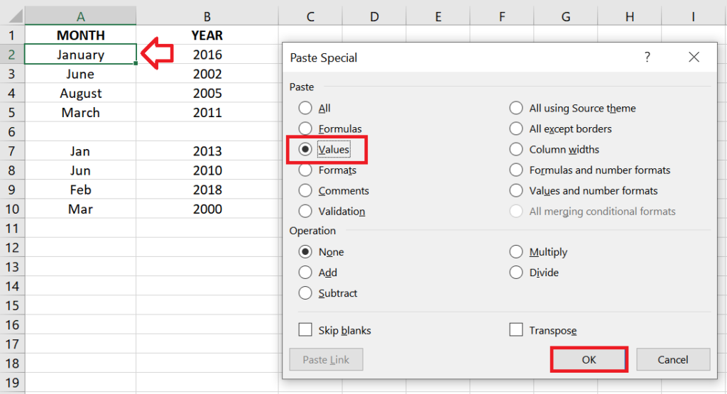
7. Go back to your original sheet. Click on the first cell in your Month column and press CTRL + ALT + V. The Paste Special menu will appear. Select Values and click OK.
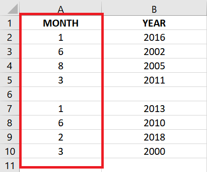
8. That’s it! Your month should now be in numerical format.
Using the DATE() Formula
Once our Month and Year columns resemble the image below, we have completed the data prep.
We will now proceed to the main course – the actual conversion of month and year to date.
1. Add another column beside YEAR. We can name it DAY.
In this column, enter the number you intend to set as the day for the dates. It could be any number from 1 to 31.
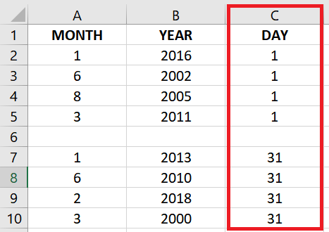
In my example above, I’ve added the first and last day of the month as my days.
2. Next, add another column after DAY. We can name it DATE.
This is where we’ll add the DATE() formulas to generate the dates based on the month, day, and year specified.
3. In cell D2, add this formula:
=DATE(B2, A2, C2)
Don’t worry if you have sorted your fields in a different order. You can change the formula accordingly.
You only have to remember that the DATE() function gets the following parameters (in this order): year, month, and day.
4. Copy cell D2 to the remaining cells in the DATE column.
5. That’s it! You should now have your actual dates.
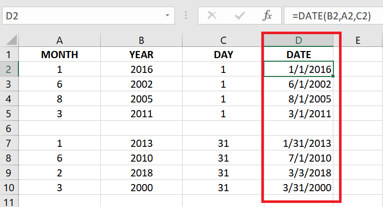
Remember to choose the number for your DAY wisely if you want to have the dates correctly reflect the Month and Year.
It may not be ideal to choose 31 as the day of the dates, considering that not all months have 31 days.
In my example above, notice that in cell D8, the result was 7/1/2010 even if the month, day, and year are 6, 31, and 2010 respectively. It should have resulted in 6/31/2010, but since this is not a valid date, Excel automatically gets the next closest day — 7/1/2010.
6. Once you’re happy with the outcome, copy the DATE column and paste it as values in your original dataset.
Steps to convert date to month and year in Excel
To reverse the process and convert the date to month and year, you can do either of the following options.
If you want to have month and year in separate columns, use the following formulas:
(Note that the sample formulas below assume that your date is in cell A2).
| MONTH | YEAR |
| =MONTH(A2) Results in the numerical value of the month. | =YEAR(A2) Results in the 4-digit value of the year. |
| =TEXT(A2, “mmm”) Results in the first three letters of the month (e.g., Jan, Feb). | =TEXT(A2, “yyyy”) Results in the 4-digit value of the year. |
| =TEXT(A2, “mmmm”) Results in the complete name of the month (e.g., January, February). | =TEXT(A2, “yy”) Results in the last two digits of the year (e.g., 22 for 2022) |
If you want to have the month and year merge and share the same column:
| MONTH AND YEAR | RESULT |
| =YEAR(A2) & “-“ & MONTH(A2) Combine the Year and Month with a dash (-). | 2022-01 |
| =MONTH(A2) & “/” & YEAR(A2) Combine the Month and Year with a slash(/). | 01/2022 |
| =TEXT(A2, “yyyymm”) Combine the Year and Month without a space or symbol in between. | 202201 |
Conclusion
Converting dates can be tricky if you’re not adept with the options available in Excel. But I hope the suggestions above will help you easily convert dates without much hassle.