Need to transform your long list of negative numbers to positive? I got you.
Whether you need to permanently convert your list of negative numbers to positive or just want to have them appear as positive numbers (but still remain negative), we have ways for that.
I would suggest going through each method so you can find the best one that fits your need.
In the latter part of this article, I’ll also show you how you can automatically transform negative numbers into positive ones using VBA and Power Query.
Change Negative Numbers to Positive in Excel (Appearance Only)
If you need to keep your numbers to stay negative and only want them to appear as positive numbers in the cells, then this method is for you.
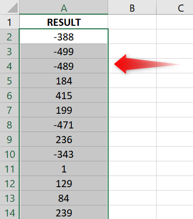
1. Highlight all cells that contain your negative numbers.
Note: It doesn’t matter if some of the cells contain positive numbers. You can include them in the selection.
2. Go to the Home tab and click the Number Format button (see the small arrow in the Number section).
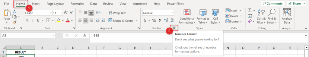
3. The Format Cells menu will appear.
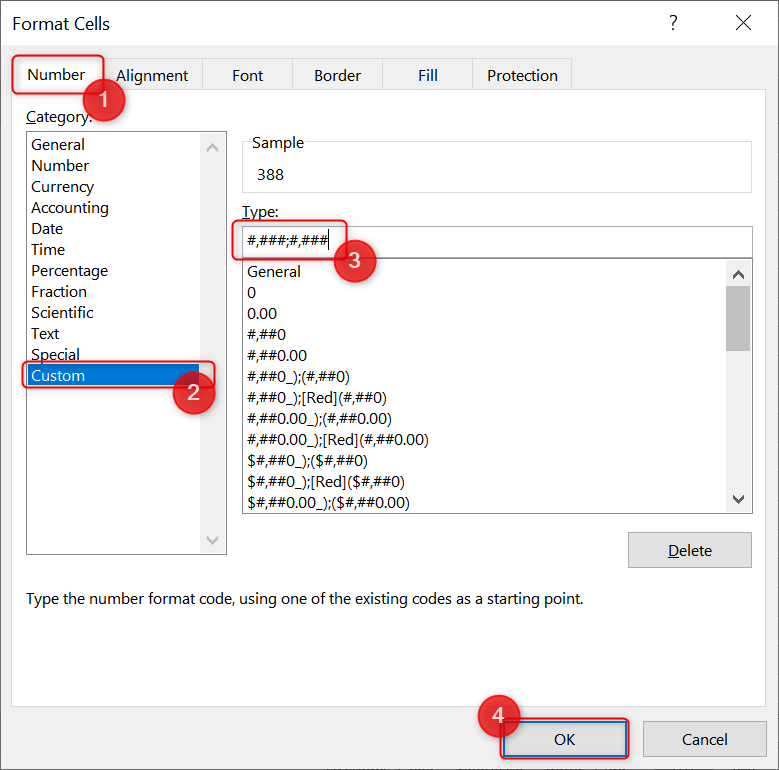
- Go to the Number tab.
- From the list of Categories, select Custom.
- Copy the following text to the Type textbox: #,###;#,###
- Once done, click OK.
The custom format we entered states that both the positive and negative numbers will have the same number formatting — no negative sign, parentheses, or any symbol to highlight the negative numbers.
4. After clicking OK, you should immediately see the selected cells all contain positive numbers.
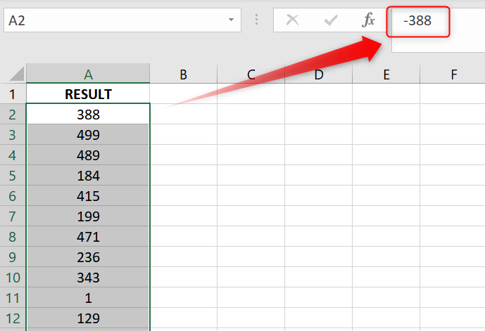
When you click on each cell and look at the formula bar, you should see that the negative numbers stay negative (but only appear positive in the cells).
Change Negative Numbers to Positive in Excel (Replace the Actual Values)
If you want to permanently replace all negative numbers with their positive counterpart, then we have two ways to do that.
Method #1: Using the Paste Special Method
Note that this method will only work best on cells that only contain negative numbers (no positive numbers in between).
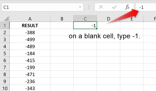
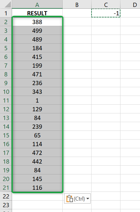
1. On a blank cell, type -1.
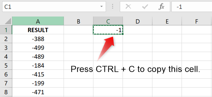
2. Select this cell and press CTRL + C to copy it.
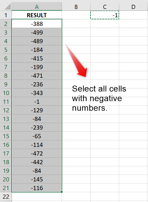
3. Select all the cells that only contain negative numbers.
Note: The cells that you select should only contain negative numbers.
If your list of numbers contains both positive and negative, please proceed to the next method as that will likely be more convenient for you.
4. Press CTRL + ALT + V to open the Paste Special menu.
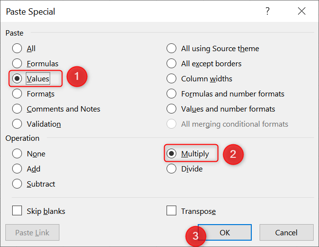
In the list of Paste options, select Values.
In the list of Operations, select Multiply and click OK.
5. And that’s it! All the negative numbers in your selected cells should now turn positive.
Method #2: By Removing All the Dashes
We all know that the dash that comes before a number signifies that a number is negative. So, one of the fastest ways to change a number from negative to positive is to remove this symbol.
To do this:
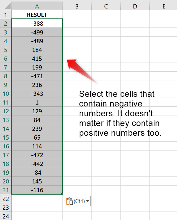
1. Highlight all the cells that contain negative numbers. It doesn’t matter if this group of cells contains positive numbers too.
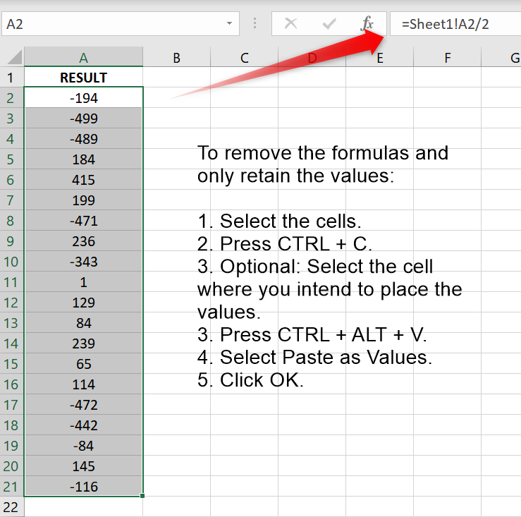
2. If these cells contain formulas, you’ll need to copy and paste them as values first.
If you like, you can paste them on a different column to preserve the cells that contain formulas.
To do this:
- Highlight the cells with numbers.
- Press CTRL + C to copy them.
- Select a cell where you’d like to paste them (it could be in the same column or in a different column)
- Press CTRL + ALT + V to open the Paste Special menu.
- From the Paste Special menu, select Values and click OK.
- And that’s it. The formulas are now removed from the cells, and only the values remain.
3. With the cells highlighted, Press CTRL + H to open the Find and Replace menu.
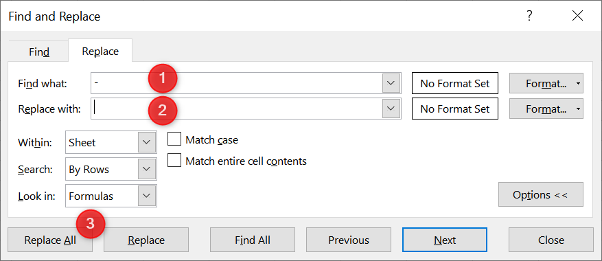
- In the Find What textbox, type a dash (-).
- Leave the Replace with textbox blank.
- Click the Replace All button.
4. And that’s it! All the negative numbers in your group of cells should now be converted to positive.
Change Negative Numbers to Positive in Excel (in a Separate Column)
If you prefer converting the negative numbers in a separate column, then you would like the following methods. With these methods, it doesn’t matter if some of the cells contain a positive number.
Method #1: Using the IF() Function
1. On a new column, type the following formula: =IF([range]>=0, [range], [range]*-1)
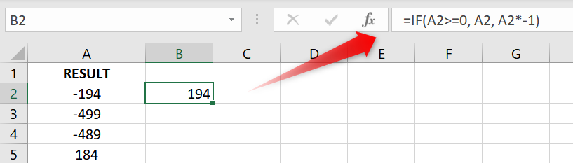
Example: =IF(A2>=0, A2, A2*-1)
What this formula does is that if it sees that the range contains a number greater than or equal to 0, it retains that value. Otherwise, it multiplies the number by -1 to get the positive value.
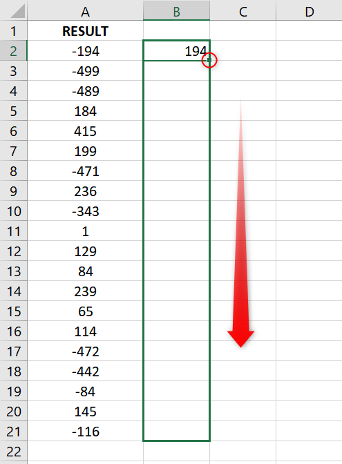
2. Drag the Fill Handle down (up to the last row in your dataset) to copy the formula to the remaining cells.
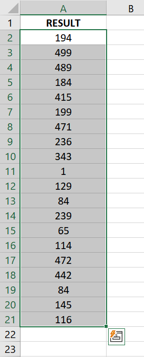
3. And that’s it! You have your negative numbers converted into positive numbers in a new column.
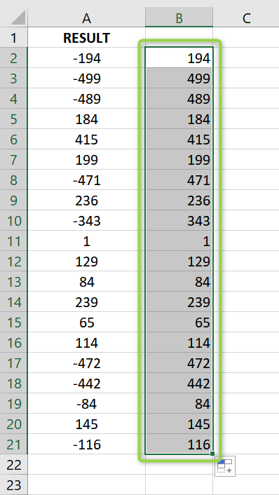
If you want, you can copy and paste this column as values to remove the formula and only retain the values.
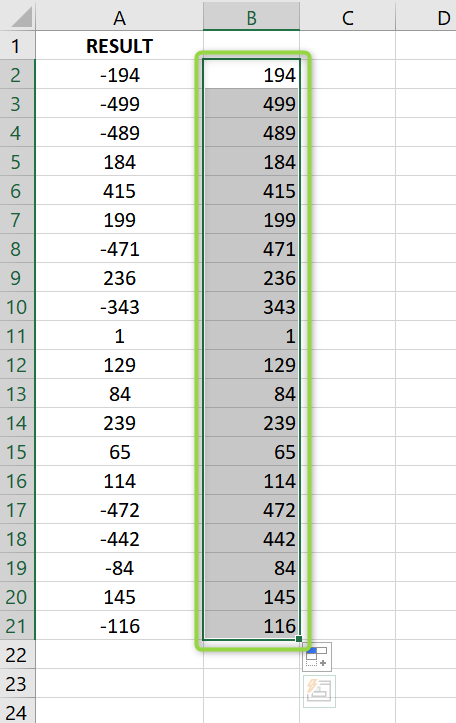
Method #2: Using the ABS() Function
1. On a new column, enter the following formula: =ABS([range])
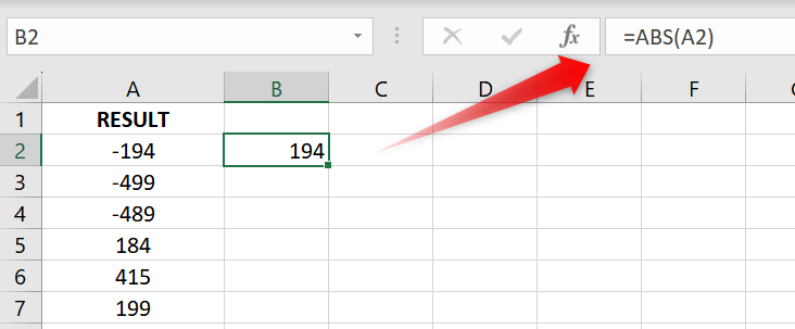
Example: =ABS(A2)
What this formula does is that it returns the absolute value of a number, that is, without the sign.
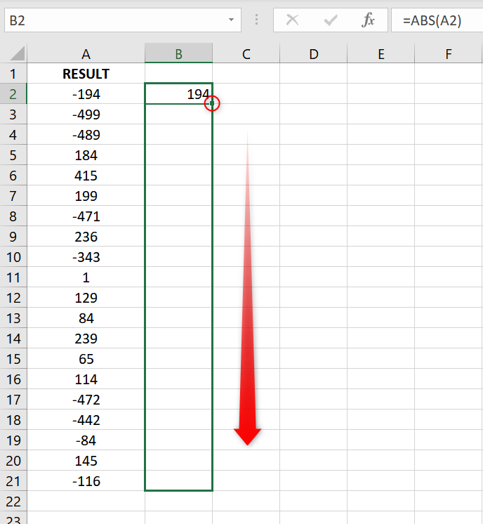
2. After entering the first formula, drag the Fill Handle down (up to the last row in the dataset).
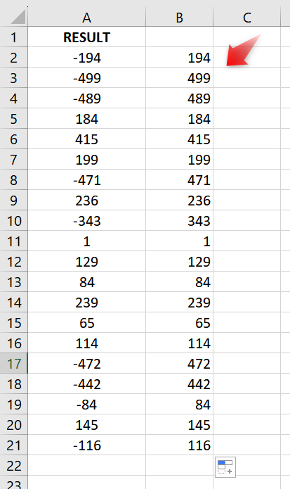
3. And that’s it! You have successfully transformed all numbers into their positive format.
Method #3: Using Flash Fill
If you don’t like formulas as much, then this method might work for you.
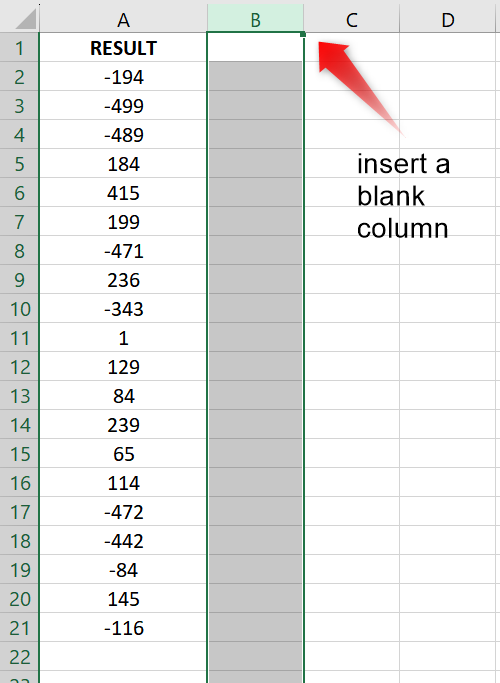
1. Insert a blank column just next to the numbers you want to convert.
IMPORTANT: This new column should be just beside your numbers. Otherwise, this method will not work.
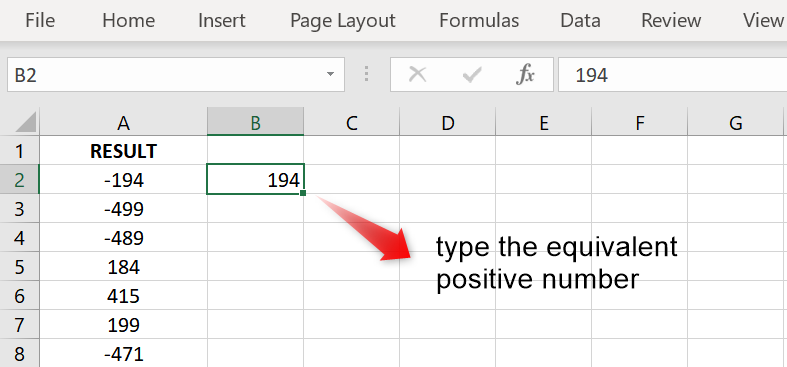
2. In the first data row, type the output you want to generate.
So, in our case, type the positive equivalent of the negative number in the original column (as shown in the example below).
3. Next, drag the Fill Handle down (up to the last row in the dataset).
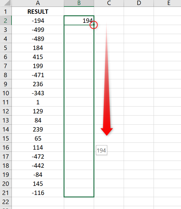
4. Notice that the number you have entered will be repeated in the remaining cells.
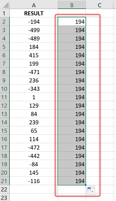
Don’t worry. This is just temporary.
5. Click the AutoFill Options button (the one that appears in the last cell).
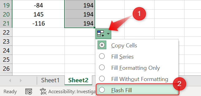
From the dropdown menu, select Flash Fill.
6. And that’s it! You should see the corresponding positive numbers in this new column.
Change Negative Numbers to Positive in Excel Using VBA
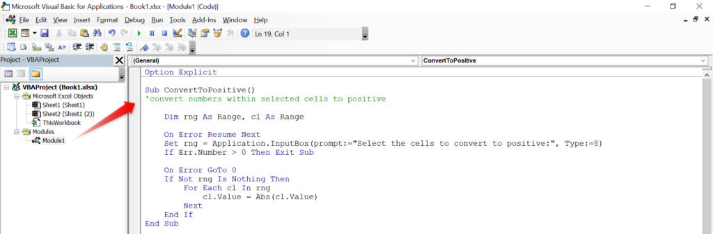
If you want to automate the process of converting negative numbers to positive ones, you can use the following code:
Option Explicit

Sub ConvertToPositive()
'convert numbers within selected cells to positive

    Dim rng As Range, cl As Range

    On Error Resume Next
    Set rng = Application.InputBox(prompt:="Select the cells to convert to positive:", Type:=8)
    If Err.Number > 0 Then Exit Sub

    On Error GoTo 0
    If Not rng Is Nothing Then
        For Each cl In rng
            cl.Value = Abs(cl.Value)
        Next
    End If
End Sub
To add this code to your workbook:
1. With your file open, press ALT + F11 to open the VBA Editor.
2. Go to the Insert tab and select Module.

To run the code, click anywhere inside the code to move the cursor there and click the Play button on top.
A prompt will then appear asking you to select the cells containing numbers that you’d like to convert to positive.
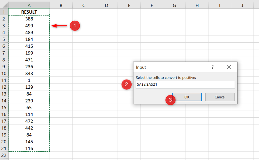
- Go back to your worksheet and select the cells you want to convert.
- The address of the cells that you have selected should appear in the input box.
- If you’re happy with it, click OK.
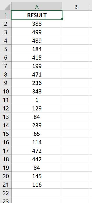
And that’s it! All the numbers inside the selected cells should now become positive.
Change Negative Numbers to Positive in Excel Using the Power Query
If you prefer a Power Query over a VBA Code to automate the number conversion, you can do the following:
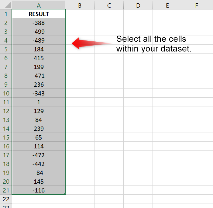
1. Select all the cells within your entire dataset.
2. Go to the Data tab and click the From Table/Range option under the Get & Transform Data section.

3. The Power Query will load for a few seconds. Then, a prompt will appear to confirm the range of cells that will be included in the table.
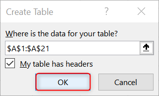
Click OK to continue.
4. The Power Query Editor will appear.
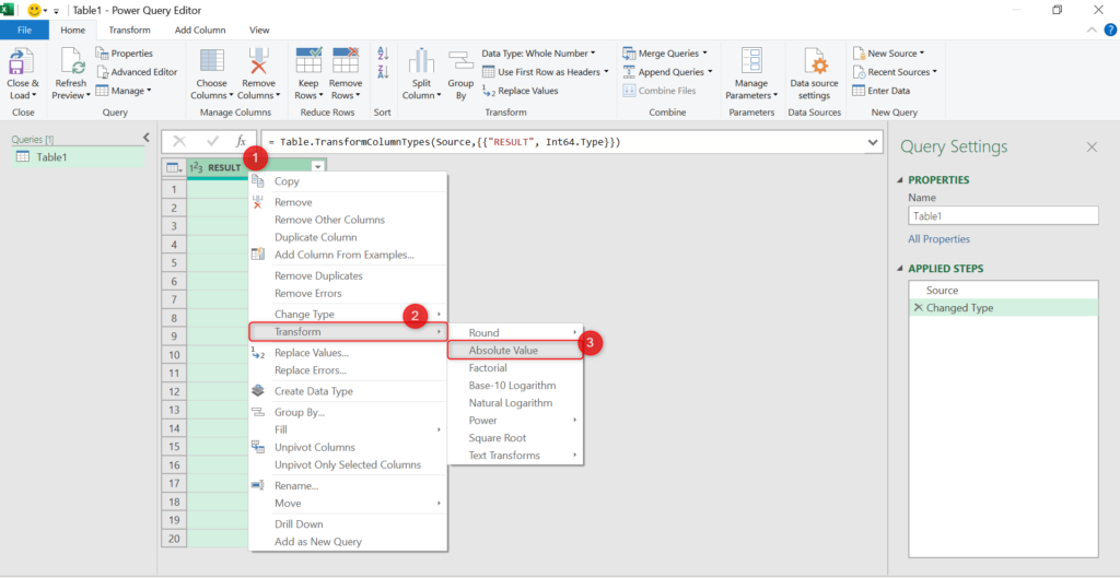
Right-click the header of the field that contains your negative numbers.
From the dropdown list that appears, select Transform >> Absolute Value.
5. And that’s it! All the negative numbers should be converted to positive ones.
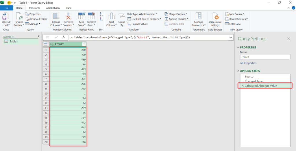
You should also see “Calculated Absolute Value” as one of the Applied Steps.
The next time you run this power query, the selected field will automatically be converted to contain positive values.
Also, if you wonder how to convert different types of data within Excel, you can check these articles:
Conclusion
As you can see, there are a lot of ways to convert negative numbers to their positive equivalent in Excel. I hope you were able to find the solution that you were looking for.