How to Sort by Last Name in Excel

Sorting information in Excel helps with classifying your data and arranging it in ascending or descending patterns. This tutorial walks you through several ways of sorting the data, including sorting statically or using formulas to keep the datasets dynamic.

Using the Sort Function to Sort by Last Name in Excel 

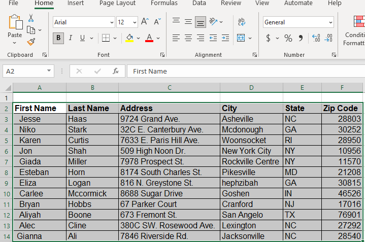
1. Highlight the table that you wish to Sort.

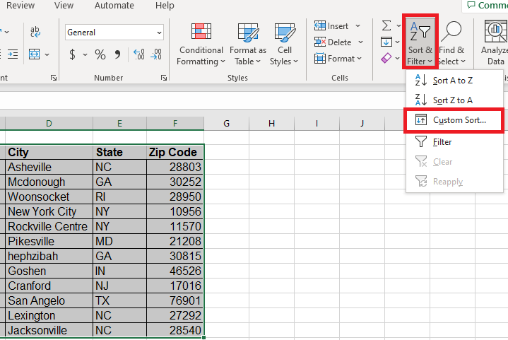
2. Click the down arrow in the Sort and Filter Group, and then choose “Custom Sort…“

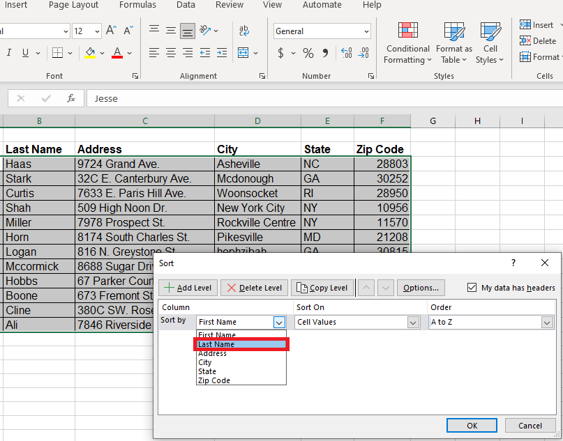
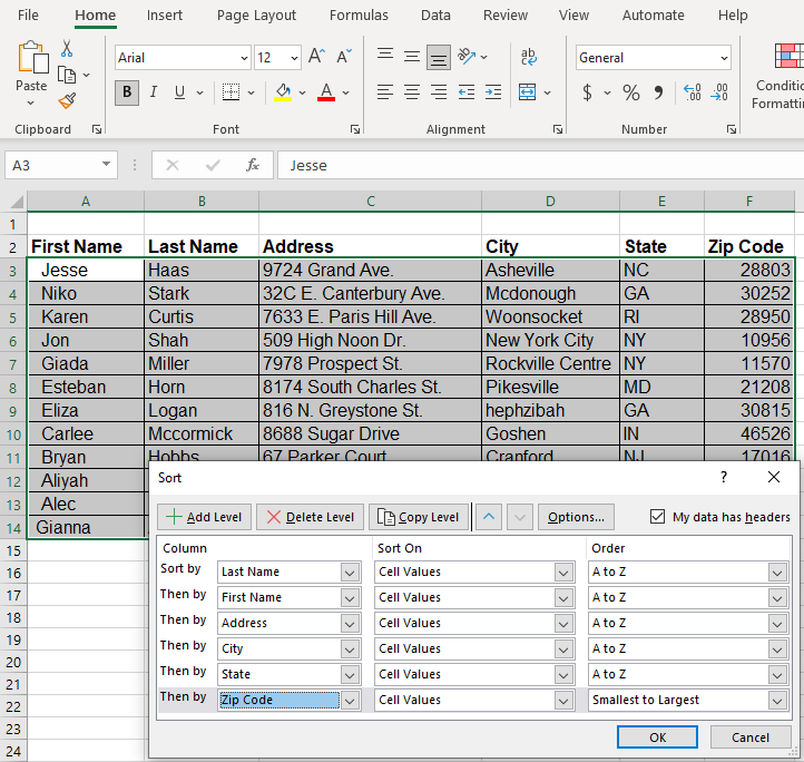
3. The Sort dialog box opens, click the down arrow next to Sort By, and click “Last Name.”

4. Next, click the “Add Level” button and select “First Name.”

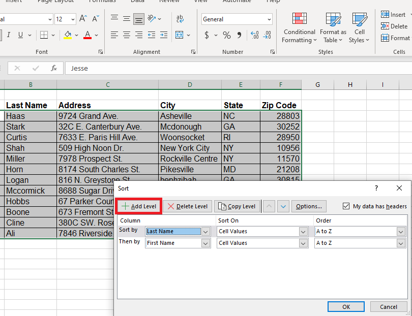
5. Continue adding levels for each data type in the table, so your Sort By dialog box looks similar to this.

Sometimes the data used in a sort is not separated into its own column, so you need to extract the data and place it into another column before sorting it.

Using Text to Columns to Sort by Last Name in Excel

1. Create a new column for the Last Name field.

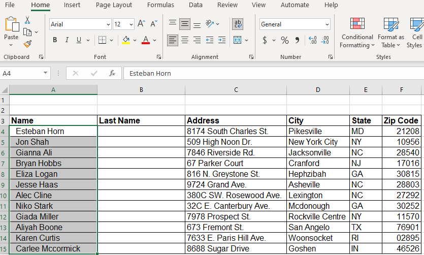
2. Highlight the Name column.

3. Click the Data tab and then select “Text to Columns” in the Data Tools Group.

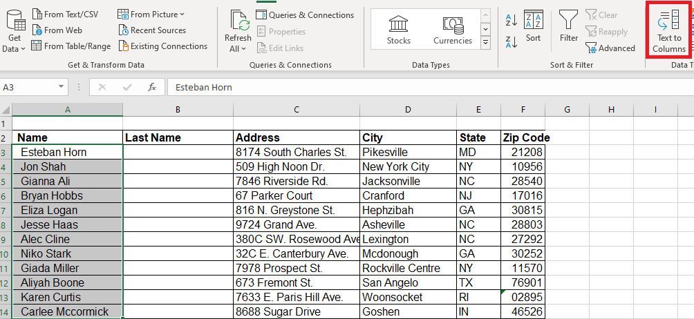
4. The Text to Columns dialog box appears.

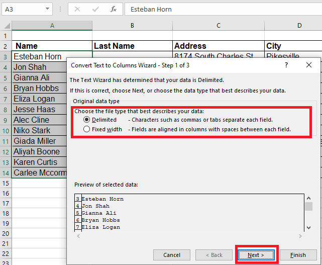
5. Choose whether your data is “Fixed Width” or “Delimited.” Make sure you are happy with the preview of your data and then click the “Next” button.

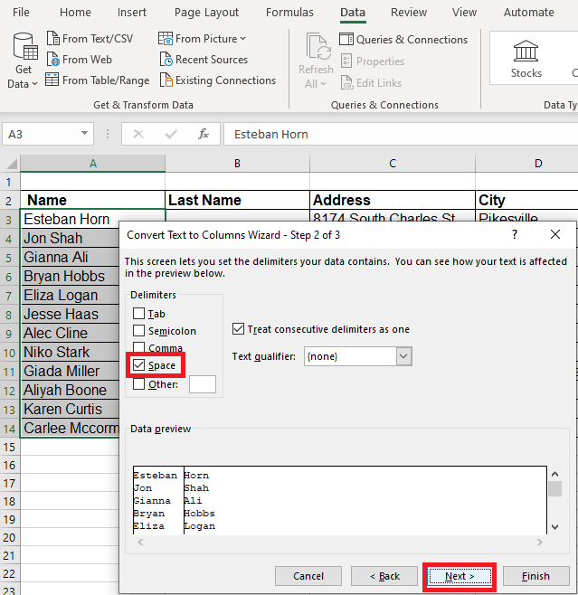
6. Click the checkbox next to “Space,” to let Excel know that a space separates the first name from the last name. Make sure the data preview shows a vertical line between the first and last names and click the “Next” button.

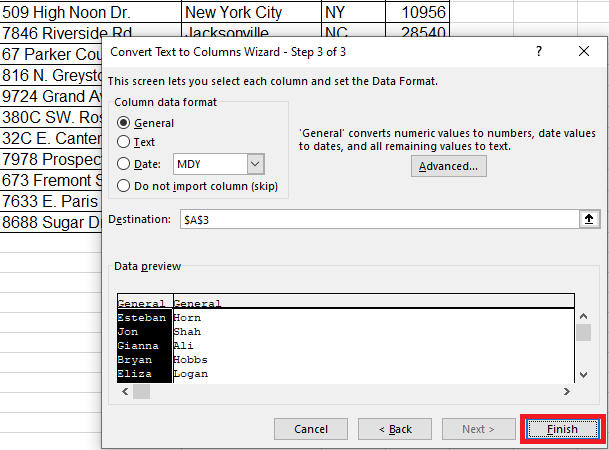
7. The next screen allows you to set the formatting for your dataset.  Given that we are working with text, leave the option selected as “General” and click the “Finish” button to complete the Text to Columns Wizard.

Note: If Excel returns a message that data already exists in the original Name column, click the “OK” button to copy over it.

Using the Find and Select Function to Sort by Last Name in Excel

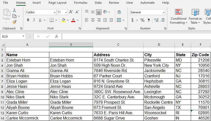
1. Insert an empty column next to the names in your data and copy the Names into it so that you have two columns with the same data.

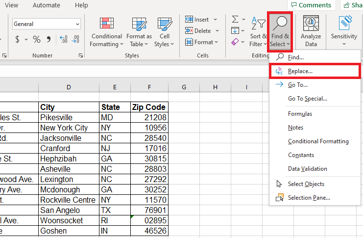
2. Select all of the data in the second column and then click on Find & Select in the Editing group of the Excel toolbar and click “Replace” to open the dialog box.

3. Type an asterisk (*) and one blank space in the “Find what:” field and leave the “Replace” field blank.

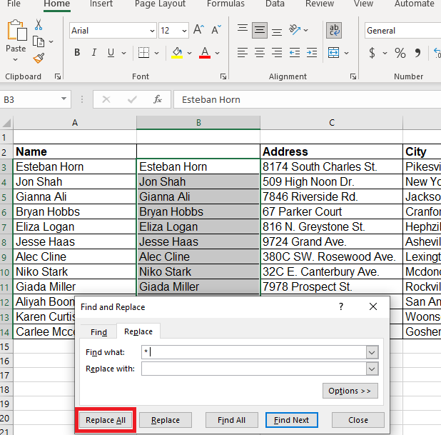
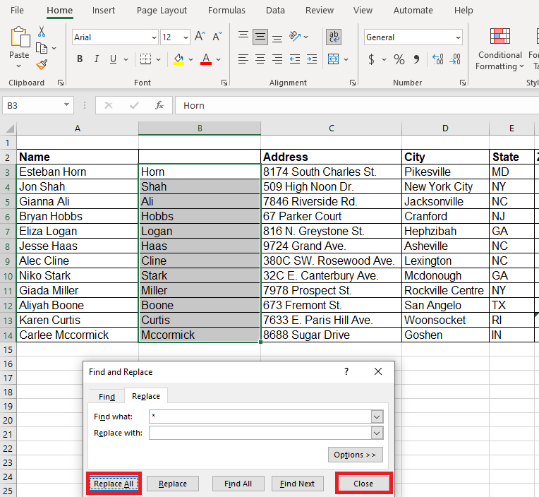
4. Tap the “Replace All” button and then close the dialog box.

Note: Using the Find and replace option in Excel is fast and easy but the only problem is that it leaves the data static. When you add names to the list, you must go back and perform Find and Replace for each new name you add to the column. So, implementing a formula into the Last Name column will save you time because you will only have to copy the formula to each new addition.

Use the LEN, RIGHT, and SEARCH Functions to Sort by Last Name in Excel

The RIGHT and LEN Functions are used to count the characters in the text string while the SEARCH function finds a specific place in a string of text, which happens to be a space in our example.

1. Insert a new column next to the column of names in your table.

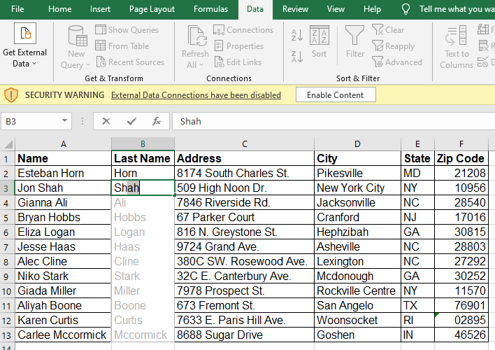
2. Type the following formula in the first cell of the new column: =RIGHT(A2,LEN(A2)-SEARCH(” “,A2,1))

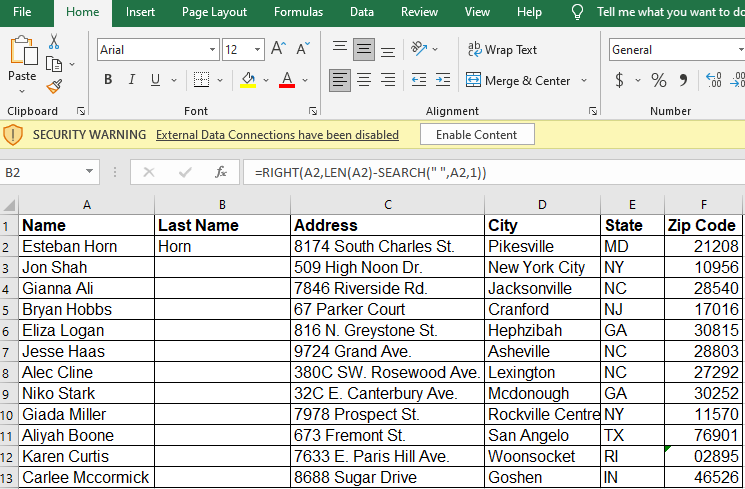
3. Copy the formula from cell B2 through the remaining cells in the column using the Fill Handle, and your new column will look similar to the image below.

Using the Flash Fill Method to Sort by Last Name in Excel

The Flash Fill concept in Excel is programmed to recognize patterns in your data and predict the patterns and fill them in without much effort from you. Here is how the Flash Fill method works in Excel.

1. Create an empty column for the Last Names in Excel.

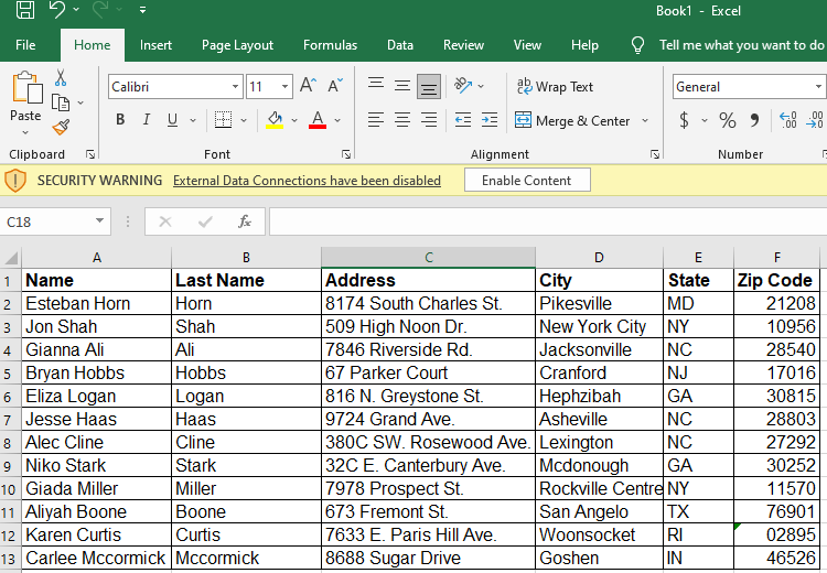
2. Type the Last Name of the first person in the dataset and then press the <ENTER> key.

3. Start typing the Last Name of the second person in the list and a list will appear for the remainder of the data set.

4. Press the <ENTER> key again and the last names appear in the column.

Using Power Query to Sort by Last Name in Excel

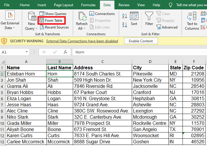
1. Click any cell in your data.
2. Click the “From Table” icon in the Get & Transform Group.

2. The Create Table dialog box appears. Make sure that you select the entire table and press the “OK” button.

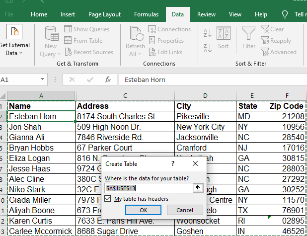
Note: If Excel returns a Security Message, press “OK” to accept it.

4. The Power Query Editor opens.

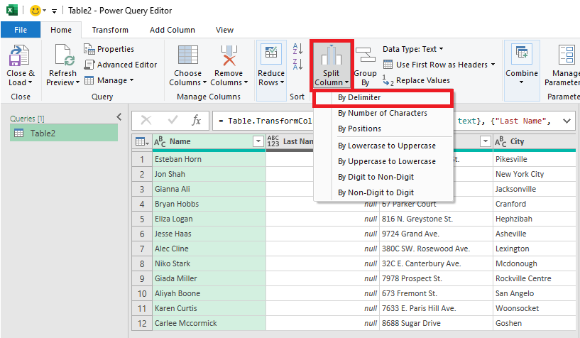
5. Click the down arrow next to “Split Columns,” and tap the “By Delimiter” option.

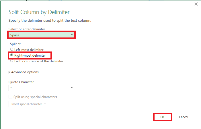
6. The Split by Delimiter dialog box opens. Select “Space” as the delimiter and then select “Right-most delimiter” in the “Split at” section and then press the “OK” button.

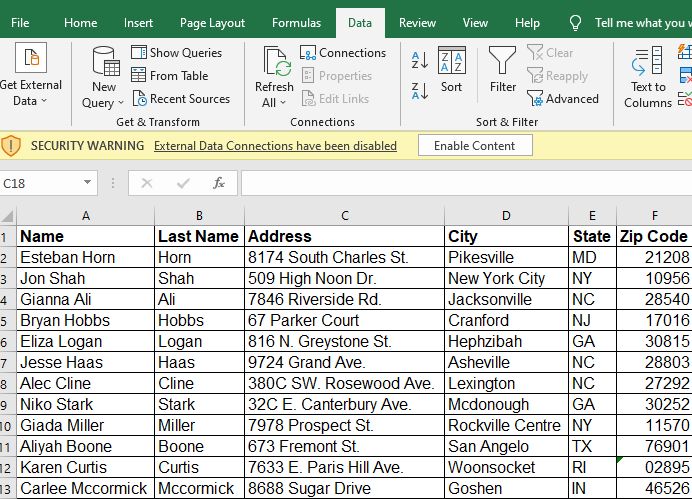
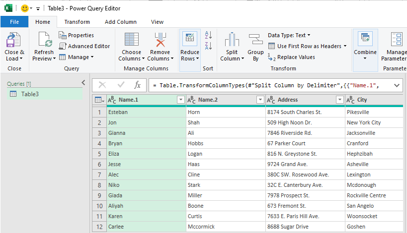
7. The Power Query splits the Last Name from the First Name and places the Last Names in a new column.

8. Click “Close & Load” in the upper left-hand corner of the Power Query dialog box.

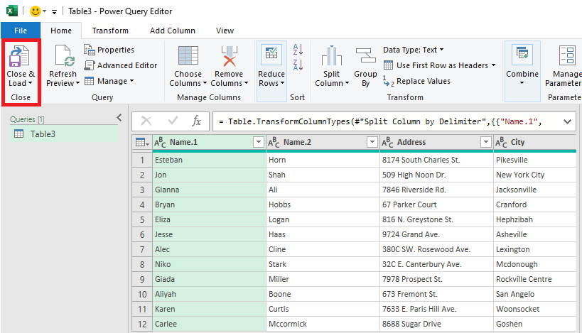
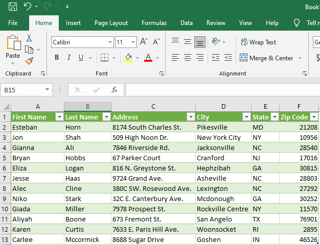
9. The dialog box closes and the new table appears in the Excel sheet.

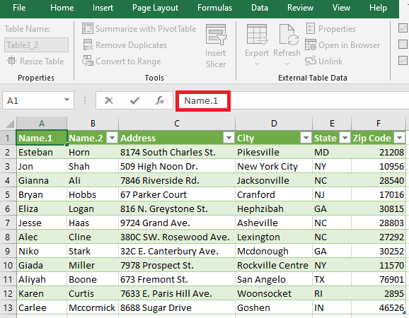
10. You can rename the columns previously changed by the Power Query. Click the Name.1 cell and insert a new name in the Formula Bar. Repeat the process for the Name.2 cell. We will choose “First Name” and “Last Name” for our example.

Now that you have built a Power Query, the next time you need to separate First Names from Last Names, you can just connect your power query to the file and run the query to complete the process.

Conclusion

Hopefully, this tutorial taught you some different ways to separate and sort data and inspires you to continue learning the different aspects of working with data in Excel.